Linear regression is a simple yet powerful technique for predicting the values of variables based on other variables. It is often used for modeling relationships between two or more continuous variables, such as the relationship between income and age, or the relationship between weight and height. Likewise, linear regression can be used to predict continuous outcomes such as price or quantity demand, based on other variables that are known to influence these outcomes.
In order to train a linear regression model, we need to define a cost function and an optimizer. The cost function is used to measure how well our model fits the data, while the optimizer decides which direction to move in order to improve this fit.
While in the previous tutorial you learned how we can make simple predictions with only a linear regression forward pass, here you’ll train a linear regression model and update its learning parameters using PyTorch. Particularly, you’ll learn:
- How you can build a simple linear regression model from scratch in PyTorch.
- How you can apply a simple linear regression model on a dataset.
- How a simple linear regression model can be trained on a single learnable parameter.
- How a simple linear regression model can be trained on two learnable parameters.
Kick-start your project with my book Deep Learning with PyTorch. It provides self-study tutorials with working code.
So, let’s get started.

Training a Linear Regression Model in PyTorch.
Picture by Ryan Tasto. Some rights reserved.
Overview
This tutorial is in four parts; they are
- Preparing Data
- Building the Model and Loss Function
- Training the Model for a Single Parameter
- Training the Model for Two Parameters
Preparing Data
Let’s import a few libraries we’ll use in this tutorial and make some data for our experiments.
|
1 2 3 |
import torch import numpy as np import matplotlib.pyplot as plt |
We will use synthetic data to train the linear regression model. We’ll initialize a variable X with values from $-5$ to $5$ and create a linear function that has a slope of $-5$. Note that this function will be estimated by our trained model later.
|
1 2 3 4 |
... # Creating a function f(X) with a slope of -5 X = torch.arange(-5, 5, 0.1).view(-1, 1) func = -5 * X |
Also, we’ll see how our data looks like in a line plot, using matplotlib.
|
1 2 3 4 5 6 7 8 |
... # Plot the line in red with grids plt.plot(X.numpy(), func.numpy(), 'r', label='func') plt.xlabel('x') plt.ylabel('y') plt.legend() plt.grid('True', color='y') plt.show() |
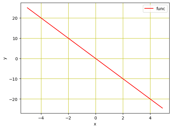
Plot of the linear function
As we need to simulate the real data we just created, let’s add some Gaussian noise to it in order to create noisy data of the same size as $X$, keeping the value of standard deviation at 0.4. This will be done by using torch.randn(X.size()).
|
1 2 3 |
... # Adding Gaussian noise to the function f(X) and saving it in Y Y = func + 0.4 * torch.randn(X.size()) |
Now, let’s visualize these data points using below lines of code.
|
1 2 3 4 5 6 7 8 |
# Plot and visualizing the data points in blue plt.plot(X.numpy(), Y.numpy(), 'b+', label='Y') plt.plot(X.numpy(), func.numpy(), 'r', label='func') plt.xlabel('x') plt.ylabel('y') plt.legend() plt.grid('True', color='y') plt.show() |
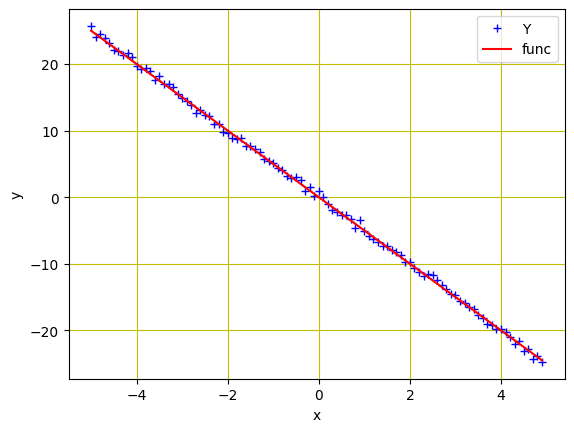
Data points and the linear function
Putting all together, the following is the complete code.
|
1 2 3 4 5 6 7 8 9 10 11 12 13 14 15 16 17 18 19 |
import torch import numpy as np import matplotlib.pyplot as plt # Creating a function f(X) with a slope of -5 X = torch.arange(-5, 5, 0.1).view(-1, 1) func = -5 * X # Adding Gaussian noise to the function f(X) and saving it in Y Y = func + 0.4 * torch.randn(X.size()) # Plot and visualizing the data points in blue plt.plot(X.numpy(), Y.numpy(), 'b+', label='Y') plt.plot(X.numpy(), func.numpy(), 'r', label='func') plt.xlabel('x') plt.ylabel('y') plt.legend() plt.grid('True', color='y') plt.show() |
Building the Model and Loss Function
We created the data to feed into the model, next we’ll build a forward function based on a simple linear regression equation. Note that we’ll build the model to train only a single parameter ($w$) here. Later, in the sext section of the tutorial, we’ll add the bias and train the model for two parameters ($w$ and $b$). The function for the forward pass of the model is defined as follows:
|
1 2 3 |
# defining the function for forward pass for prediction def forward(x): return w * x |
In training steps, we’ll need a criterion to measure the loss between the original and the predicted data points. This information is crucial for gradient descent optimization operations of the model and updated after every iteration in order to calculate the gradients and minimize the loss. Usually, linear regression is used for continuous data where Mean Square Error (MSE) effectively calculates the model loss. Therefore MSE metric is the criterion function we use here.
|
1 2 3 |
# evaluating data points with Mean Square Error. def criterion(y_pred, y): return torch.mean((y_pred - y) ** 2) |
Want to Get Started With Deep Learning with PyTorch?
Take my free email crash course now (with sample code).
Click to sign-up and also get a free PDF Ebook version of the course.
Training the Model for a Single Parameter
With all these preparations, we are ready for model training. First, the parameter $w$ need to be initialized randomly, for example, to the value $-10$.
|
1 |
w = torch.tensor(-10.0, requires_grad=True) |
Next, we’ll define the learning rate or the step size, an empty list to store the loss after each iteration, and the number of iterations we want our model to train for. While the step size is set at 0.1, we train the model for 20 iterations per epochs.
|
1 2 3 |
step_size = 0.1 loss_list = [] iter = 20 |
When below lines of code is executed, the forward() function takes an input and generates a prediction. The criterian() function calculates the loss and stores it in loss variable. Based on the model loss, the backward() method computes the gradients and w.data stores the updated parameters.
|
1 2 3 4 5 6 7 8 9 10 11 12 13 14 15 |
for i in range (iter): # making predictions with forward pass Y_pred = forward(X) # calculating the loss between original and predicted data points loss = criterion(Y_pred, Y) # storing the calculated loss in a list loss_list.append(loss.item()) # backward pass for computing the gradients of the loss w.r.t to learnable parameters loss.backward() # updateing the parameters after each iteration w.data = w.data - step_size * w.grad.data # zeroing gradients after each iteration w.grad.data.zero_() # priting the values for understanding print('{},\t{},\t{}'.format(i, loss.item(), w.item())) |
The output of the model training is printed as under. As you can see, model loss reduces after every iteration and the trainable parameter (which in this case is $w$) is updated.
|
1 2 3 4 5 6 7 8 9 10 11 12 13 14 15 16 17 18 19 20 |
0, 207.40255737304688, -1.6875505447387695 1, 92.3563003540039, -7.231954097747803 2, 41.173553466796875, -3.5338361263275146 3, 18.402894973754883, -6.000481128692627 4, 8.272472381591797, -4.355228900909424 5, 3.7655599117279053, -5.452612400054932 6, 1.7604843378067017, -4.7206573486328125 7, 0.8684477210044861, -5.208871364593506 8, 0.471589595079422, -4.883232593536377 9, 0.2950323224067688, -5.100433826446533 10, 0.21648380160331726, -4.955560684204102 11, 0.1815381944179535, -5.052190780639648 12, 0.16599132120609283, -4.987738609313965 13, 0.15907476842403412, -5.030728340148926 14, 0.15599775314331055, -5.002054214477539 15, 0.15462875366210938, -5.021179676055908 16, 0.15401971340179443, -5.008423328399658 17, 0.15374873578548431, -5.016931533813477 18, 0.15362821519374847, -5.011256694793701 19, 0.15357455611228943, -5.015041828155518 |
Let’s also visualize via the plot to see how the loss reduces.
|
1 2 3 4 5 6 7 |
# Plotting the loss after each iteration plt.plot(loss_list, 'r') plt.tight_layout() plt.grid('True', color='y') plt.xlabel("Epochs/Iterations") plt.ylabel("Loss") plt.show() |
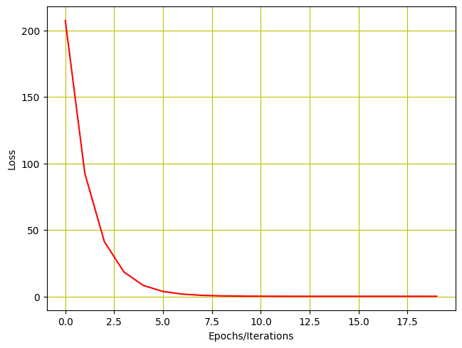
Training loss vs epochs
Putting everything together, the following is the complete code:
|
1 2 3 4 5 6 7 8 9 10 11 12 13 14 15 16 17 18 19 20 21 22 23 24 25 26 27 28 29 30 31 32 33 34 35 36 37 38 39 40 41 42 43 44 45 |
import torch import numpy as np import matplotlib.pyplot as plt X = torch.arange(-5, 5, 0.1).view(-1, 1) func = -5 * X Y = func + 0.4 * torch.randn(X.size()) # defining the function for forward pass for prediction def forward(x): return w * x # evaluating data points with Mean Square Error def criterion(y_pred, y): return torch.mean((y_pred - y) ** 2) w = torch.tensor(-10.0, requires_grad=True) step_size = 0.1 loss_list = [] iter = 20 for i in range (iter): # making predictions with forward pass Y_pred = forward(X) # calculating the loss between original and predicted data points loss = criterion(Y_pred, Y) # storing the calculated loss in a list loss_list.append(loss.item()) # backward pass for computing the gradients of the loss w.r.t to learnable parameters loss.backward() # updateing the parameters after each iteration w.data = w.data - step_size * w.grad.data # zeroing gradients after each iteration w.grad.data.zero_() # priting the values for understanding print('{},\t{},\t{}'.format(i, loss.item(), w.item())) # Plotting the loss after each iteration plt.plot(loss_list, 'r') plt.tight_layout() plt.grid('True', color='y') plt.xlabel("Epochs/Iterations") plt.ylabel("Loss") plt.show() |
Training the Model for Two Parameters
Let’s also add bias $b$ to our model and train it for two parameters. First we need to change the forward function to as follows.
|
1 2 3 |
# defining the function for forward pass for prediction def forward(x): return w * x + b |
As we have two parameters $w$ and $b$, we need to initialize both to some random values, such as below.
|
1 2 |
w = torch.tensor(-10.0, requires_grad = True) b = torch.tensor(-20.0, requires_grad = True) |
While all the other code for training will remain the same as before, we’ll only have to make a few changes for two learnable parameters.
Keeping learning rate at 0.1, lets train our model for two parameters for 20 iterations/epochs.
|
1 2 3 4 5 6 7 8 9 10 11 12 13 14 15 16 17 18 19 20 21 |
step_size = 0.1 loss_list = [] iter = 20 for i in range (iter): # making predictions with forward pass Y_pred = forward(X) # calculating the loss between original and predicted data points loss = criterion(Y_pred, Y) # storing the calculated loss in a list loss_list.append(loss.item()) # backward pass for computing the gradients of the loss w.r.t to learnable parameters loss.backward() # updateing the parameters after each iteration w.data = w.data - step_size * w.grad.data b.data = b.data - step_size * b.grad.data # zeroing gradients after each iteration w.grad.data.zero_() b.grad.data.zero_() # priting the values for understanding print('{}, \t{}, \t{}, \t{}'.format(i, loss.item(), w.item(), b.item())) |
Here is what we get for output.
|
1 2 3 4 5 6 7 8 9 10 11 12 13 14 15 16 17 18 19 20 |
0, 598.0744018554688, -1.8875503540039062, -16.046640396118164 1, 344.6290283203125, -7.2590203285217285, -12.802828788757324 2, 203.6309051513672, -3.6438119411468506, -10.261493682861328 3, 122.82559204101562, -6.029742240905762, -8.19227409362793 4, 75.30597686767578, -4.4176344871521, -6.560757637023926 5, 46.759193420410156, -5.476595401763916, -5.2394232749938965 6, 29.318675994873047, -4.757054805755615, -4.19294548034668 7, 18.525297164916992, -5.2265238761901855, -3.3485677242279053 8, 11.781207084655762, -4.90494441986084, -2.677760124206543 9, 7.537606239318848, -5.112729549407959, -2.1378984451293945 10, 4.853880405426025, -4.968738555908203, -1.7080869674682617 11, 3.1505300998687744, -5.060482025146484, -1.3627978563308716 12, 2.0666630268096924, -4.99583625793457, -1.0874838829040527 13, 1.3757448196411133, -5.0362019538879395, -0.8665863275527954 14, 0.9347621202468872, -5.007069110870361, -0.6902718544006348 15, 0.6530535817146301, -5.024737358093262, -0.5489290356636047 16, 0.4729837477207184, -5.011539459228516, -0.43603143095970154 17, 0.3578317165374756, -5.0192131996154785, -0.34558138251304626 18, 0.28417202830314636, -5.013190746307373, -0.27329811453819275 19, 0.23704445362091064, -5.01648473739624, -0.2154112160205841 |
Similarly we can plot the loss history.
|
1 2 3 4 5 6 7 |
# Plotting the loss after each iteration plt.plot(loss_list, 'r') plt.tight_layout() plt.grid('True', color='y') plt.xlabel("Epochs/Iterations") plt.ylabel("Loss") plt.show() |
And here is how the plot for the loss looks like.
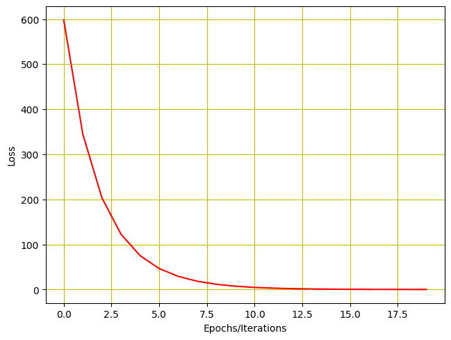
History of loss for training with two parameters
Putting everything together, this is the complete code.
|
1 2 3 4 5 6 7 8 9 10 11 12 13 14 15 16 17 18 19 20 21 22 23 24 25 26 27 28 29 30 31 32 33 34 35 36 37 38 39 40 41 42 43 44 45 46 47 48 |
import torch import numpy as np import matplotlib.pyplot as plt X = torch.arange(-5, 5, 0.1).view(-1, 1) func = -5 * X Y = func + 0.4 * torch.randn(X.size()) # defining the function for forward pass for prediction def forward(x): return w * x + b # evaluating data points with Mean Square Error. def criterion(y_pred, y): return torch.mean((y_pred - y) ** 2) w = torch.tensor(-10.0, requires_grad=True) b = torch.tensor(-20.0, requires_grad=True) step_size = 0.1 loss_list = [] iter = 20 for i in range (iter): # making predictions with forward pass Y_pred = forward(X) # calculating the loss between original and predicted data points loss = criterion(Y_pred, Y) # storing the calculated loss in a list loss_list.append(loss.item()) # backward pass for computing the gradients of the loss w.r.t to learnable parameters loss.backward() # updateing the parameters after each iteration w.data = w.data - step_size * w.grad.data b.data = b.data - step_size * b.grad.data # zeroing gradients after each iteration w.grad.data.zero_() b.grad.data.zero_() # priting the values for understanding print('{}, \t{}, \t{}, \t{}'.format(i, loss.item(), w.item(), b.item())) # Plotting the loss after each iteration plt.plot(loss_list, 'r') plt.tight_layout() plt.grid('True', color='y') plt.xlabel("Epochs/Iterations") plt.ylabel("Loss") plt.show() |
Summary
In this tutorial you learned how you can build and train a simple linear regression model in PyTorch. Particularly, you learned.
- How you can build a simple linear regression model from scratch in PyTorch.
- How you can apply a simple linear regression model on a dataset.
- How a simple linear regression model can be trained on a single learnable parameter.
- How a simple linear regression model can be trained on two learnable parameters.
Get Started on Deep Learning with PyTorch!

Learn how to build deep learning models
...using the newly released PyTorch 2.0 library
Discover how in my new Ebook:
Deep Learning with PyTorch
It provides self-study tutorials with hundreds of working code to turn you from a novice to expert. It equips you with
tensor operation, training, evaluation, hyperparameter optimization,
and much more...


I love seeing examples like this. So often we go straight to the largest and most complicated models. A linear regression is extremely powerful so so many problems. Not to mention linear regression is interpretable while deep neural nets are not. I think for the majority of problems could have a preliminary step where we apply regression methods and evaluate the learning and predictions. Great job.
Thank you for the feedback and support Stephen! We greatly appreciate it!