Training a Single Output Multilinear Regression Model in PyTorch

By Muhammad Asad Iqbal Khan on April 8, 2023 in Deep Learning with PyTorch 0

A neural network architecture is built with hundreds of neurons where each of them takes in multiple inputs to perform a multilinear regression operation for prediction. In the previous tutorials, we built a single output multilinear regression model that used only a forward function for prediction.

In this tutorial, we’ll add optimizer to our single output multilinear regression model and perform backpropagation to reduce the loss of the model. Particularly, we’ll demonstrate:

How to build a single output multilinear regression model in PyTorch.
How PyTorch built-in packages can be used to create complicated models.
How to train a single output multilinear regression model with mini-batch gradient descent in PyTorch.

Kick-start your project with my book Deep Learning with PyTorch. It provides self-study tutorials with working code.

Let’s get started.

Training a Single Output Multilinear Regression Model in PyTorch.
Picture by Bruno Nascimento. Some rights reserved.

Overview

This tutorial is in three parts; they are

Preparing Data for Prediction
Using Linear Class for Multilinear Regression
Visualize the Results

Build the Dataset Class

Just like previous tutorials, we’ll create a sample dataset to perform our experiments on. Our data class includes a dataset constructor, a getter __getitem__() to fetch the data samples, and __len__() function to get the length of the created data. Here is how it looks like.

import torch
from torch.utils.data import Dataset

# Creating the dataset class
class Data(Dataset):
    # Constructor
    def __init__(self):
        self.x = torch.zeros(40, 2)
        self.x[:, 0] = torch.arange(-2, 2, 0.1)
        self.x[:, 1] = torch.arange(-2, 2, 0.1)
        self.w = torch.tensor([[1.0], [1.0]])
        self.b = 1
        self.func = torch.mm(self.x, self.w) + self.b    
        self.y = self.func + 0.2 * torch.randn((self.x.shape[0],1))
        self.len = self.x.shape[0]
    # Getter
    def __getitem__(self, index):          
        return self.x[index], self.y[index] 
    # getting data length
    def __len__(self):
        return self.len

import torch

from torch.utils.data import Dataset

# Creating the dataset class

class Data(Dataset):

# Constructor

def __init__(self):

self.x = torch.zeros(40, 2)

self.x[:, 0] = torch.arange(-2, 2, 0.1)

self.x[:, 1] = torch.arange(-2, 2, 0.1)

self.w = torch.tensor([[1.0], [1.0]])

self.b = 1

self.func = torch.mm(self.x, self.w) + self.b

self.y = self.func + 0.2 * torch.randn((self.x.shape[0],1))

self.len = self.x.shape[0]

# Getter

def __getitem__(self, index):

return self.x[index], self.y[index]

# getting data length

def __len__(self):

return self.len

With this, we can easily create the dataset object.

# Creating dataset object
data_set = Data()

1 2	# Creating dataset object data_set = Data()

Want to Get Started With Deep Learning with PyTorch?

Take my free email crash course now (with sample code).

Click to sign-up and also get a free PDF Ebook version of the course.

Build the Model Class

Now that we have the dataset, let’s build a custom multilinear regression model class. As discussed in the previous tutorial, we define a class and make it a subclass of nn.Module. As a result, the class inherits all the methods and attributes from the latter.

...
# Creating a custom Multiple Linear Regression Model
class MultipleLinearRegression(torch.nn.Module):
    # Constructor
    def __init__(self, input_dim, output_dim):
        super().__init__()
        self.linear = torch.nn.Linear(input_dim, output_dim)
    # Prediction
    def forward(self, x):
        y_pred = self.linear(x)
        return y_pred

...

# Creating a custom Multiple Linear Regression Model

class MultipleLinearRegression(torch.nn.Module):

# Constructor

def __init__(self, input_dim, output_dim):

super().__init__()

self.linear = torch.nn.Linear(input_dim, output_dim)

# Prediction

def forward(self, x):

y_pred = self.linear(x)

return y_pred

We’ll create a model object with an input size of 2 and output size of 1. Moreover, we can print out all model parameters using the method parameters().

...
# Creating the model object
MLR_model = MultipleLinearRegression(2,1)
print("The parameters: ", list(MLR_model.parameters()))

...

# Creating the model object

MLR_model = MultipleLinearRegression(2,1)

print("The parameters: ", list(MLR_model.parameters()))

Here’s what the output looks like.

The parameters:  [Parameter containing:
tensor([[ 0.2236, -0.0123]], requires_grad=True), Parameter containing:
tensor([0.5534], requires_grad=True)]

The parameters: [Parameter containing:

tensor([[ 0.2236, -0.0123]], requires_grad=True), Parameter containing:

tensor([0.5534], requires_grad=True)]

In order to train our multilinear regression model, we also need to define the optimizer and loss criterion. We’ll employ stochastic gradient descent optimizer and mean square error loss for the model. We’ll keep the learning rate at 0.1.

# defining the model optimizer
optimizer = torch.optim.SGD(MLR_model.parameters(), lr=0.1)
# defining the loss criterion
criterion = torch.nn.MSELoss()

# defining the model optimizer

optimizer = torch.optim.SGD(MLR_model.parameters(), lr=0.1)

# defining the loss criterion

criterion = torch.nn.MSELoss()

Train the Model with Mini-Batch Gradient Descent

Before we start the training process, let’s load up our data into the DataLoader and define the batch size for the training.

from torch.utils.data import DataLoader

# Creating the dataloader
train_loader = DataLoader(dataset=data_set, batch_size=2)

from torch.utils.data import DataLoader

# Creating the dataloader

train_loader = DataLoader(dataset=data_set, batch_size=2)

We’ll start the training and let the process continue for 20 epochs, using the same for-loop as in our previous tutorial.

# Train the model
Loss = []
epochs = 20
for epoch in range(epochs):
    for x,y in train_loader:
        y_pred = MLR_model(x)
        loss = criterion(y_pred, y)
        Loss.append(loss.item())
        optimizer.zero_grad()
        loss.backward()
        optimizer.step()   
    print(f"epoch = {epoch}, loss = {loss}")
print("Done training!")

# Train the model

Loss = []

epochs = 20

for epoch in range(epochs):

for x,y in train_loader:

y_pred = MLR_model(x)

loss = criterion(y_pred, y)

Loss.append(loss.item())

optimizer.zero_grad()

loss.backward()

optimizer.step()

print(f"epoch = {epoch}, loss = {loss}")

print("Done training!")

In the training loop above, the loss is reported in each epoch. You should see the output similar to the following:

epoch = 0, loss = 0.06849382817745209
epoch = 1, loss = 0.07729718089103699
epoch = 2, loss = 0.0755983218550682
epoch = 3, loss = 0.07591515779495239
epoch = 4, loss = 0.07585576921701431
epoch = 5, loss = 0.07586675882339478
epoch = 6, loss = 0.07586495578289032
epoch = 7, loss = 0.07586520910263062
epoch = 8, loss = 0.07586534321308136
epoch = 9, loss = 0.07586508244276047
epoch = 10, loss = 0.07586508244276047
epoch = 11, loss = 0.07586508244276047
epoch = 12, loss = 0.07586508244276047
epoch = 13, loss = 0.07586508244276047
epoch = 14, loss = 0.07586508244276047
epoch = 15, loss = 0.07586508244276047
epoch = 16, loss = 0.07586508244276047
epoch = 17, loss = 0.07586508244276047
epoch = 18, loss = 0.07586508244276047
epoch = 19, loss = 0.07586508244276047
Done training!

epoch = 0, loss = 0.06849382817745209

epoch = 1, loss = 0.07729718089103699

epoch = 2, loss = 0.0755983218550682

epoch = 3, loss = 0.07591515779495239

epoch = 4, loss = 0.07585576921701431

epoch = 5, loss = 0.07586675882339478

epoch = 6, loss = 0.07586495578289032

epoch = 7, loss = 0.07586520910263062

epoch = 8, loss = 0.07586534321308136

epoch = 9, loss = 0.07586508244276047

epoch = 10, loss = 0.07586508244276047

epoch = 11, loss = 0.07586508244276047

epoch = 12, loss = 0.07586508244276047

epoch = 13, loss = 0.07586508244276047

epoch = 14, loss = 0.07586508244276047

epoch = 15, loss = 0.07586508244276047

epoch = 16, loss = 0.07586508244276047

epoch = 17, loss = 0.07586508244276047

epoch = 18, loss = 0.07586508244276047

epoch = 19, loss = 0.07586508244276047

Done training!

This training loop is typical in PyTorch. You will reuse it very often in future projects.

Plot the Graph

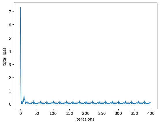
Lastly, let’s plot the graph to visualize how the loss decreases during the training process and converge to a certain point.

...
import matplotlib.pyplot as plt

# Plot the graph for epochs and loss
plt.plot(Loss)
plt.xlabel("Iterations ")
plt.ylabel("total loss ")
plt.show()

...

import matplotlib.pyplot as plt

# Plot the graph for epochs and loss

plt.plot(Loss)

plt.xlabel("Iterations ")

plt.ylabel("total loss ")

plt.show()

Loss during training

Putting everything together, the following is the complete code.

# Importing libraries and packages
import numpy as np
import torch
import matplotlib.pyplot as plt
from torch.utils.data import Dataset, DataLoader

torch.manual_seed(42)

# Creating the dataset class
class Data(Dataset):
    # Constructor
    def __init__(self):
        self.x = torch.zeros(40, 2)
        self.x[:, 0] = torch.arange(-2, 2, 0.1)
        self.x[:, 1] = torch.arange(-2, 2, 0.1)
        self.w = torch.tensor([[1.0], [1.0]])
        self.b = 1
        self.func = torch.mm(self.x, self.w) + self.b    
        self.y = self.func + 0.2 * torch.randn((self.x.shape[0],1))
        self.len = self.x.shape[0]
    # Getter
    def __getitem__(self, index):          
        return self.x[index], self.y[index] 
    # getting data length
    def __len__(self):
        return self.len

# Creating dataset object
data_set = Data()

# Creating a custom Multiple Linear Regression Model
class MultipleLinearRegression(torch.nn.Module):
    # Constructor
    def __init__(self, input_dim, output_dim):
        super().__init__()
        self.linear = torch.nn.Linear(input_dim, output_dim)
    # Prediction
    def forward(self, x):
        y_pred = self.linear(x)
        return y_pred

# Creating the model object
MLR_model = MultipleLinearRegression(2,1)
# defining the model optimizer
optimizer = torch.optim.SGD(MLR_model.parameters(), lr=0.1)
# defining the loss criterion
criterion = torch.nn.MSELoss()
# Creating the dataloader
train_loader = DataLoader(dataset=data_set, batch_size=2)

# Train the model
Loss = []
epochs = 20
for epoch in range(epochs):
    for x,y in train_loader:
        y_pred = MLR_model(x)
        loss = criterion(y_pred, y)
        Loss.append(loss.item())
        optimizer.zero_grad()
        loss.backward()
        optimizer.step()   
    print(f"epoch = {epoch}, loss = {loss}")
print("Done training!")

# Plot the graph for epochs and loss
plt.plot(Loss)
plt.xlabel("Iterations ")
plt.ylabel("total loss ")
plt.show()

# Importing libraries and packages

import numpy as np

import torch

import matplotlib.pyplot as plt

from torch.utils.data import Dataset, DataLoader

torch.manual_seed(42)

# Creating the dataset class

class Data(Dataset):

# Constructor

def __init__(self):

self.x = torch.zeros(40, 2)

self.x[:, 0] = torch.arange(-2, 2, 0.1)

self.x[:, 1] = torch.arange(-2, 2, 0.1)

self.w = torch.tensor([[1.0], [1.0]])

self.b = 1

self.func = torch.mm(self.x, self.w) + self.b

self.y = self.func + 0.2 * torch.randn((self.x.shape[0],1))

self.len = self.x.shape[0]

# Getter

def __getitem__(self, index):

return self.x[index], self.y[index]

# getting data length

def __len__(self):

return self.len

# Creating dataset object

data_set = Data()

# Creating a custom Multiple Linear Regression Model

class MultipleLinearRegression(torch.nn.Module):

# Constructor

def __init__(self, input_dim, output_dim):

super().__init__()

self.linear = torch.nn.Linear(input_dim, output_dim)

# Prediction

def forward(self, x):

y_pred = self.linear(x)

return y_pred

# Creating the model object

MLR_model = MultipleLinearRegression(2,1)

# defining the model optimizer

optimizer = torch.optim.SGD(MLR_model.parameters(), lr=0.1)

# defining the loss criterion

criterion = torch.nn.MSELoss()

# Creating the dataloader

train_loader = DataLoader(dataset=data_set, batch_size=2)

# Train the model

Loss = []

epochs = 20

for epoch in range(epochs):

for x,y in train_loader:

y_pred = MLR_model(x)

loss = criterion(y_pred, y)

Loss.append(loss.item())

optimizer.zero_grad()

loss.backward()

optimizer.step()

print(f"epoch = {epoch}, loss = {loss}")

print("Done training!")

# Plot the graph for epochs and loss

plt.plot(Loss)

plt.xlabel("Iterations ")

plt.ylabel("total loss ")

plt.show()

Summary

In this tutorial you learned how to build a single output multilinear regression model in PyTorch. Particularly, you learned:

How to build a single output multilinear regression model in PyTorch.
How PyTorch built-in packages can be used to create complicated models.
How to train a single output multilinear regression model with mini-batch gradient descent in PyTorch.

Navigation

Training a Single Output Multilinear Regression Model in PyTorch

Overview

Build the Dataset Class

Want to Get Started With Deep Learning with PyTorch?

Build the Model Class

Train the Model with Mini-Batch Gradient Descent

Plot the Graph

Summary

Get Started on Deep Learning with PyTorch!

Learn how to build deep learning models

Kick-start your deep learning journey with hands-on exercises

More On This Topic

No comments yet.

Leave a Reply Click here to cancel reply.