Mini-batch gradient descent is a variant of gradient descent algorithm that is commonly used to train deep learning models. The idea behind this algorithm is to divide the training data into batches, which are then processed sequentially. In each iteration, we update the weights of all the training samples belonging to a particular batch together. This process is repeated with different batches until the whole training data has been processed. Compared to batch gradient descent, the main benefit of this approach is that it can reduce computation time and memory usage significantly as compared to processing all training samples in one shot.
DataLoader is a module in PyTorch that loads and preprocesses data for deep learning models. It can be used to load the data from a file, or to generate synthetic data.
In this tutorial, we will introduce you to the concept of mini-batch gradient descent. You will also get to know how to implement it with PyTorch DataLoader. Particularly, we’ll cover:
- Implementation of Mini-Batch Gradient Descent in PyTorch.
- The concept of DataLoader in PyTorch and how we can load the data with it.
- The difference between Stochastic Gradient Descent and Mini-Batch Gradient Descent.
- How to implement Stochastic Gradient Descent with PyTorch DataLoader.
- How to implement Mini-Batch Gradient Descent with PyTorch DataLoader.
Kick-start your project with my book Deep Learning with PyTorch. It provides self-study tutorials with working code.
Let’s get started.

Mini-Batch Gradient Descent and DataLoader in PyTorch.
Picture by Yannis Papanastasopoulos. Some rights reserved.
Overview
This tutorial is in six parts; they are
- DataLoader in PyTorch
- Preparing Data and the Linear Regression Model
- Build Dataset and DataLoader Class
- Training with Stochastic Gradient Descent and DataLoader
- Training with Mini-Batch Gradient Descent and DataLoader
- Plotting Graphs for Comparison
DataLoader in PyTorch
It all starts with loading the data when you plan to build a deep learning pipeline to train a model. The more complex the data, the more difficult it becomes to load it into the pipeline. PyTorch DataLoader is a handy tool offering numerous options not only to load the data easily, but also helps to apply data augmentation strategies, and iterate over samples in larger datasets. You can import DataLoader class from torch.utils.data, as follows.
|
1 |
from torch.utils.data import DataLoader |
There are several parameters in the DataLoader class, we’ll only discuss about dataset and batch_size. The dataset is the first parameter you’ll find in the DataLoader class and it loads your data into the pipeline. The second parameter is the batch_size which indicates the number of training examples processed in one iteration.
|
1 |
DataLoader(dataset, batch_size=n) |
Preparing Data and the Linear Regression Model
Let’s reuse the same linear regression data as we produced in the previous tutorial:
|
1 2 3 4 5 6 7 8 9 10 |
import torch import numpy as np import matplotlib.pyplot as plt # Creating a function f(X) with a slope of -5 X = torch.arange(-5, 5, 0.1).view(-1, 1) func = -5 * X # Adding Gaussian noise to the function f(X) and saving it in Y Y = func + 0.4 * torch.randn(X.size()) |
Same as in the previous tutorial, we initialized a variable X with values ranging from $-5$ to $5$, and created a linear function with a slope of $-5$. Then, Gaussian noise is added to create the variable Y.
We can plot the data using matplotlib to visualize the pattern:
|
1 2 3 4 5 6 7 8 9 |
... # Plot and visualizing the data points in blue plt.plot(X.numpy(), Y.numpy(), 'b+', label='Y') plt.plot(X.numpy(), func.numpy(), 'r', label='func') plt.xlabel('x') plt.ylabel('y') plt.legend() plt.grid('True', color='y') plt.show() |
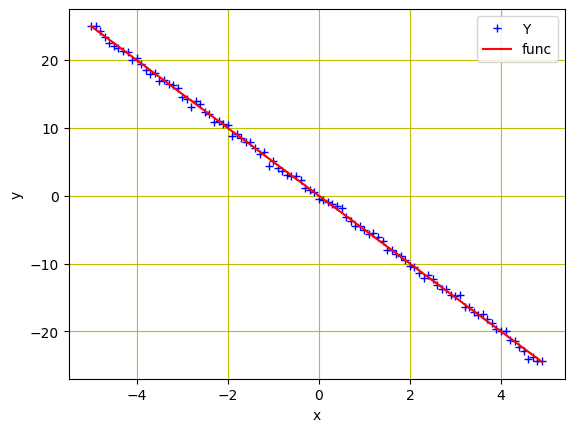
Data points for regression model
Next, we’ll build a forward function based on a simple linear regression equation. We’ll train the model for two parameters ($w$ and $b$). So, let’s define a function for the forward pass of the model as well as a loss criterion function (MSE loss). The parameter variables w and b will be defined outside of the function:
|
1 2 3 4 5 6 7 8 |
... # defining the function for forward pass for prediction def forward(x): return w * x + b # evaluating data points with Mean Square Error (MSE) def criterion(y_pred, y): return torch.mean((y_pred - y) ** 2) |
Want to Get Started With Deep Learning with PyTorch?
Take my free email crash course now (with sample code).
Click to sign-up and also get a free PDF Ebook version of the course.
Build Dataset and DataLoader Class
Let’s build our Dataset and DataLoader classes. The Dataset class allows us to build custom datasets and apply various transforms on them. The DataLoader class, on the other hand, is used to load the datasets into the pipeline for model training. They are created as follows.
|
1 2 3 4 5 6 7 8 9 10 11 12 13 14 15 16 17 |
# Creating our dataset class class Build_Data(Dataset): # Constructor def __init__(self): self.x = torch.arange(-5, 5, 0.1).view(-1, 1) self.y = -5 * X self.len = self.x.shape[0] # Getting the data def __getitem__(self, index): return self.x[index], self.y[index] # Getting length of the data def __len__(self): return self.len # Creating DataLoader object dataset = Build_Data() train_loader = DataLoader(dataset = dataset, batch_size = 1) |
Training with Stochastic Gradient Descent and DataLoader
When the batch size is set to one, the training algorithm is referred to as stochastic gradient descent. Likewise, when the batch size is greater than one but less than the size of the entire training data, the training algorithm is known as mini-batch gradient descent. For simplicity, let’s train with stochastic gradient descent and DataLoader.
As before, we’ll randomly initialize the trainable parameters $w$ and $b$, define other parameters such as learning rate or step size, create an empty list to store the loss, and set the number of epochs of training.
|
1 2 3 4 5 6 |
w = torch.tensor(-10.0, requires_grad = True) b = torch.tensor(-20.0, requires_grad = True) step_size = 0.1 loss_SGD = [] n_iter = 20 |
In SGD, we just need to pick one sample from the dataset in each iteration of training. Hence a simple for loop with a forward and backward pass is all we needed:
|
1 2 3 4 5 6 7 8 9 10 11 12 13 14 15 16 17 |
for i in range (n_iter): # calculating loss as in the beginning of an epoch and storing it y_pred = forward(X) loss_SGD.append(criterion(y_pred, Y).tolist()) for x, y in train_loader: # making a prediction in forward pass y_hat = forward(x) # calculating the loss between original and predicted data points loss = criterion(y_hat, y) # backward pass for computing the gradients of the loss w.r.t to learnable parameters loss.backward() # updating the parameters after each iteration w.data = w.data - step_size * w.grad.data b.data = b.data - step_size * b.grad.data # zeroing gradients after each iteration w.grad.data.zero_() b.grad.data.zero_() |
Putting everything together, the following is a complete code to train the model, namely, w and b:
|
1 2 3 4 5 6 7 8 9 10 11 12 13 14 15 16 17 18 19 20 21 22 23 24 25 26 27 28 29 30 31 32 33 34 35 36 37 38 39 40 41 42 43 44 45 46 47 48 49 50 51 52 53 54 55 56 57 58 59 60 61 62 |
import matplotlib.pyplot as plt import torch from torch.utils.data import Dataset from torch.utils.data import DataLoader torch.manual_seed(42) # Creating a function f(X) with a slope of -5 X = torch.arange(-5, 5, 0.1).view(-1, 1) func = -5 * X # Adding Gaussian noise to the function f(X) and saving it in Y Y = func + 0.4 * torch.randn(X.size()) w = torch.tensor(-10.0, requires_grad = True) b = torch.tensor(-20.0, requires_grad = True) # defining the function for forward pass for prediction def forward(x): return w * x + b # evaluating data points with Mean Square Error (MSE) def criterion(y_pred, y): return torch.mean((y_pred - y) ** 2) # Creating our dataset class class Build_Data(Dataset): # Constructor def __init__(self): self.x = torch.arange(-5, 5, 0.1).view(-1, 1) self.y = -5 * X self.len = self.x.shape[0] # Getting the data def __getitem__(self, index): return self.x[index], self.y[index] # Getting length of the data def __len__(self): return self.len # Creating DataLoader object dataset = Build_Data() train_loader = DataLoader(dataset=dataset, batch_size=1) step_size = 0.1 loss_SGD = [] n_iter = 20 for i in range (n_iter): # calculating loss as in the beginning of an epoch and storing it y_pred = forward(X) loss_SGD.append(criterion(y_pred, Y).tolist()) for x, y in train_loader: # making a prediction in forward pass y_hat = forward(x) # calculating the loss between original and predicted data points loss = criterion(y_hat, y) # backward pass for computing the gradients of the loss w.r.t to learnable parameters loss.backward() # updating the parameters after each iteration w.data = w.data - step_size * w.grad.data b.data = b.data - step_size * b.grad.data # zeroing gradients after each iteration w.grad.data.zero_() b.grad.data.zero_() |
Training with Mini-Batch Gradient Descent and DataLoader
Moving one step further, we’ll train our model with mini-batch gradient descent and DataLoader. We’ll set various batch sizes for training, i.e., batch sizes of 10 and 20. Training with batch size of 10 is as follows:
|
1 2 3 4 5 6 7 8 9 10 11 12 13 14 15 16 17 18 19 20 21 22 23 24 25 26 27 |
... train_loader_10 = DataLoader(dataset=dataset, batch_size=10) w = torch.tensor(-10.0, requires_grad=True) b = torch.tensor(-20.0, requires_grad=True) step_size = 0.1 loss_MBGD_10 = [] iter = 20 for i in range (iter): # calculating loss as in the beginning of an epoch and storing it y_pred = forward(X) loss_MBGD_10.append(criterion(y_pred, Y).tolist()) for x, y in train_loader_10: # making a prediction in forward pass y_hat = forward(x) # calculating the loss between original and predicted data points loss = criterion(y_hat, y) # backward pass for computing the gradients of the loss w.r.t to learnable parameters loss.backward() # updating the parameters after each iteration w.data = w.data - step_size * w.grad.data b.data = b.data - step_size * b.grad.data # zeroing gradients after each iteration w.grad.data.zero_() b.grad.data.zero_() |
And, here is how we’ll implement the same with batch size of 20:
|
1 2 3 4 5 6 7 8 9 10 11 12 13 14 15 16 17 18 19 20 21 22 23 24 25 26 27 |
... train_loader_20 = DataLoader(dataset=dataset, batch_size=20) w = torch.tensor(-10.0, requires_grad=True) b = torch.tensor(-20.0, requires_grad=True) step_size = 0.1 loss_MBGD_20 = [] iter = 20 for i in range(iter): # calculating loss as in the beginning of an epoch and storing it y_pred = forward(X) loss_MBGD_20.append(criterion(y_pred, Y).tolist()) for x, y in train_loader_20: # making a prediction in forward pass y_hat = forward(x) # calculating the loss between original and predicted data points loss = criterion(y_hat, y) # backward pass for computing the gradients of the loss w.r.t to learnable parameters loss.backward() # updating the parameters after each iteration w.data = w.data - step_size * w.grad.data b.data = b.data - step_size * b.grad.data # zeroing gradients after each iteration w.grad.data.zero_() b.grad.data.zero_() |
Putting all together, the following is the complete code:
|
1 2 3 4 5 6 7 8 9 10 11 12 13 14 15 16 17 18 19 20 21 22 23 24 25 26 27 28 29 30 31 32 33 34 35 36 37 38 39 40 41 42 43 44 45 46 47 48 49 50 51 52 53 54 55 56 57 58 59 60 61 62 63 64 65 66 67 68 69 70 71 72 73 74 75 76 77 78 79 80 81 82 83 84 85 86 87 88 |
import matplotlib.pyplot as plt import torch from torch.utils.data import Dataset from torch.utils.data import DataLoader torch.manual_seed(42) # Creating a function f(X) with a slope of -5 X = torch.arange(-5, 5, 0.1).view(-1, 1) func = -5 * X # Adding Gaussian noise to the function f(X) and saving it in Y Y = func + 0.4 * torch.randn(X.size()) w = torch.tensor(-10.0, requires_grad=True) b = torch.tensor(-20.0, requires_grad=True) # defining the function for forward pass for prediction def forward(x): return w * x + b # evaluating data points with Mean Square Error (MSE) def criterion(y_pred, y): return torch.mean((y_pred - y) ** 2) # Creating our dataset class class Build_Data(Dataset): # Constructor def __init__(self): self.x = torch.arange(-5, 5, 0.1).view(-1, 1) self.y = -5 * X self.len = self.x.shape[0] # Getting the data def __getitem__(self, index): return self.x[index], self.y[index] # Getting length of the data def __len__(self): return self.len # Creating DataLoader object dataset = Build_Data() train_loader_10 = DataLoader(dataset=dataset, batch_size=10) step_size = 0.1 loss_MBGD_10 = [] iter = 20 for i in range(n_iter): # calculating loss as in the beginning of an epoch and storing it y_pred = forward(X) loss_MBGD_10.append(criterion(y_pred, Y).tolist()) for x, y in train_loader_10: # making a prediction in forward pass y_hat = forward(x) # calculating the loss between original and predicted data points loss = criterion(y_hat, y) # backward pass for computing the gradients of the loss w.r.t to learnable parameters loss.backward() # updateing the parameters after each iteration w.data = w.data - step_size * w.grad.data b.data = b.data - step_size * b.grad.data # zeroing gradients after each iteration w.grad.data.zero_() b.grad.data.zero_() train_loader_20 = DataLoader(dataset=dataset, batch_size=20) # Reset w and b w = torch.tensor(-10.0, requires_grad=True) b = torch.tensor(-20.0, requires_grad=True) loss_MBGD_20 = [] for i in range(n_iter): # calculating loss as in the beginning of an epoch and storing it y_pred = forward(X) loss_MBGD_20.append(criterion(y_pred, Y).tolist()) for x, y in train_loader_20: # making a prediction in forward pass y_hat = forward(x) # calculating the loss between original and predicted data points loss = criterion(y_hat, y) # backward pass for computing the gradients of the loss w.r.t to learnable parameters loss.backward() # updating the parameters after each iteration w.data = w.data - step_size * w.grad.data b.data = b.data - step_size * b.grad.data # zeroing gradients after each iteration w.grad.data.zero_() b.grad.data.zero_() |
Plotting Graphs for Comparison
Finally, let’s visualize how the loss decreases in all the three algorithms (i.e., stochastic gradient descent, mini-batch gradient descent with batch size of 10, and with batch size of 20) during training.
|
1 2 3 4 5 6 7 |
plt.plot(loss_SGD,label = "Stochastic Gradient Descent") plt.plot(loss_MBGD_10,label = "Mini-Batch-10 Gradient Descent") plt.plot(loss_MBGD_20,label = "Mini-Batch-20 Gradient Descent") plt.xlabel('epoch') plt.ylabel('Cost/total loss') plt.legend() plt.show() |
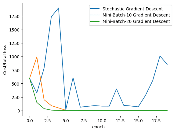
As we can see from the plot, mini-batch gradient descent can converge faster because we can make more precise update to the parameters by calculating the average loss in each step.
Putting all together, the following is the complete code:
|
1 2 3 4 5 6 7 8 9 10 11 12 13 14 15 16 17 18 19 20 21 22 23 24 25 26 27 28 29 30 31 32 33 34 35 36 37 38 39 40 41 42 43 44 45 46 47 48 49 50 51 52 53 54 55 56 57 58 59 60 61 62 63 64 65 66 67 68 69 70 71 72 73 74 75 76 77 78 79 80 81 82 83 84 85 86 87 88 89 90 91 92 93 94 95 96 97 98 99 100 101 102 103 104 105 106 107 108 109 110 111 112 113 114 115 116 117 118 119 120 121 122 |
import matplotlib.pyplot as plt import torch from torch.utils.data import Dataset from torch.utils.data import DataLoader torch.manual_seed(42) # Creating a function f(X) with a slope of -5 X = torch.arange(-5, 5, 0.1).view(-1, 1) func = -5 * X # Adding Gaussian noise to the function f(X) and saving it in Y Y = func + 0.4 * torch.randn(X.size()) w = torch.tensor(-10.0, requires_grad=True) b = torch.tensor(-20.0, requires_grad=True) # defining the function for forward pass for prediction def forward(x): return w * x + b # evaluating data points with Mean Square Error (MSE) def criterion(y_pred, y): return torch.mean((y_pred - y) ** 2) # Creating our dataset class class Build_Data(Dataset): # Constructor def __init__(self): self.x = torch.arange(-5, 5, 0.1).view(-1, 1) self.y = -5 * X self.len = self.x.shape[0] # Getting the data def __getitem__(self, index): return self.x[index], self.y[index] # Getting length of the data def __len__(self): return self.len # Creating DataLoader object dataset = Build_Data() train_loader = DataLoader(dataset=dataset, batch_size=1) step_size = 0.1 loss_SGD = [] n_iter = 20 for i in range(n_iter): # calculating loss as in the beginning of an epoch and storing it y_pred = forward(X) loss_SGD.append(criterion(y_pred, Y).tolist()) for x, y in train_loader: # making a prediction in forward pass y_hat = forward(x) # calculating the loss between original and predicted data points loss = criterion(y_hat, y) # backward pass for computing the gradients of the loss w.r.t to learnable parameters loss.backward() # updating the parameters after each iteration w.data = w.data - step_size * w.grad.data b.data = b.data - step_size * b.grad.data # zeroing gradients after each iteration w.grad.data.zero_() b.grad.data.zero_() train_loader_10 = DataLoader(dataset=dataset, batch_size=10) # Reset w and b w = torch.tensor(-10.0, requires_grad=True) b = torch.tensor(-20.0, requires_grad=True) loss_MBGD_10 = [] for i in range(n_iter): # calculating loss as in the beginning of an epoch and storing it y_pred = forward(X) loss_MBGD_10.append(criterion(y_pred, Y).tolist()) for x, y in train_loader_10: # making a prediction in forward pass y_hat = forward(x) # calculating the loss between original and predicted data points loss = criterion(y_hat, y) # backward pass for computing the gradients of the loss w.r.t to learnable parameters loss.backward() # updating the parameters after each iteration w.data = w.data - step_size * w.grad.data b.data = b.data - step_size * b.grad.data # zeroing gradients after each iteration w.grad.data.zero_() b.grad.data.zero_() train_loader_20 = DataLoader(dataset=dataset, batch_size=20) # Reset w and b w = torch.tensor(-10.0, requires_grad=True) b = torch.tensor(-20.0, requires_grad=True) loss_MBGD_20 = [] for i in range(n_iter): # calculating loss as in the beginning of an epoch and storing it y_pred = forward(X) loss_MBGD_20.append(criterion(y_pred, Y).tolist()) for x, y in train_loader_20: # making a prediction in forward pass y_hat = forward(x) # calculating the loss between original and predicted data points loss = criterion(y_hat, y) # backward pass for computing the gradients of the loss w.r.t to learnable parameters loss.backward() # updating the parameters after each iteration w.data = w.data - step_size * w.grad.data b.data = b.data - step_size * b.grad.data # zeroing gradients after each iteration w.grad.data.zero_() b.grad.data.zero_() plt.plot(loss_SGD,label="Stochastic Gradient Descent") plt.plot(loss_MBGD_10,label="Mini-Batch-10 Gradient Descent") plt.plot(loss_MBGD_20,label="Mini-Batch-20 Gradient Descent") plt.xlabel('epoch') plt.ylabel('Cost/total loss') plt.legend() plt.show() |
Summary
In this tutorial, you learned about mini-batch gradient descent, DataLoader, and their implementation in PyTorch. Particularly, you learned:
- Implementation of mini-batch gradient descent in PyTorch.
- The concept of
DataLoaderin PyTorch and how we can load the data with it. - The difference between stochastic gradient descent and mini-batch gradient descent.
- How to implement stochastic gradient descent with PyTorch
DataLoader. - How to implement mini-batch gradient descent with PyTorch
DataLoader.
Get Started on Deep Learning with PyTorch!

Learn how to build deep learning models
...using the newly released PyTorch 2.0 library
Discover how in my new Ebook:
Deep Learning with PyTorch
It provides self-study tutorials with hundreds of working code to turn you from a novice to expert. It equips you with
tensor operation, training, evaluation, hyperparameter optimization,
and much more...


No comments yet.