Gradient descent is an optimization algorithm that follows the negative gradient of an objective function in order to locate the minimum of the function.
It is a simple and effective technique that can be implemented with just a few lines of code. It also provides the basis for many extensions and modifications that can result in better performance. The algorithm also provides the basis for the widely used extension called stochastic gradient descent, used to train deep learning neural networks.
In this tutorial, you will discover how to implement gradient descent optimization from scratch.
After completing this tutorial, you will know:
Gradient descent is a general procedure for optimizing a differentiable objective function.
How to implement the gradient descent algorithm from scratch in Python.
How to apply the gradient descent algorithm to an objective function.
Kick-start your project with my new book Optimization for Machine Learning, including step-by-step tutorials and the Python source code files for all examples.
Let’s get started.
How to Implement Gradient Descent Optimization from Scratch Photo by Bernd Thaller, some rights reserved.
Tutorial Overview
This tutorial is divided into three parts; they are:
It is technically referred to as a first-order optimization algorithm as it explicitly makes use of the first-order derivative of the target objective function.
First-order methods rely on gradient information to help direct the search for a minimum …
The first-order derivative, or simply the “derivative,” is the rate of change or slope of the target function at a specific point, e.g. for a specific input.
If the target function takes multiple input variables, it is referred to as a multivariate function and the input variables can be thought of as a vector. In turn, the derivative of a multivariate target function may also be taken as a vector and is referred to generally as the “gradient.”
Gradient: First order derivative for a multivariate objective function.
The derivative or the gradient points in the direction of the steepest ascent of the target function for an input.
The gradient points in the direction of steepest ascent of the tangent hyperplane …
Specifically, the sign of the gradient tells you if the target function is increasing or decreasing at that point.
Positive Gradient: Function is increasing at that point.
Negative Gradient: Function is decreasing at that point.
Gradient descent refers to a minimization optimization algorithm that follows the negative of the gradient downhill of the target function to locate the minimum of the function.
Similarly, we may refer to gradient ascent for the maximization version of the optimization algorithm that follows the gradient uphill to the maximum of the target function.
Gradient Descent: Minimization optimization that follows the negative of the gradient to the minimum of the target function.
Gradient Ascent: Maximization optimization that follows the gradient to the maximum of the target function.
Central to gradient descent algorithms is the idea of following the gradient of the target function.
By definition, the optimization algorithm is only appropriate for target functions where the derivative function is available and can be calculated for all input values. This does not apply to all target functions, only so-called differentiable functions.
The main benefit of the gradient descent algorithm is that it is easy to implement and effective on a wide range of optimization problems.
Gradient methods are simple to implement and often perform well.
Gradient descent refers to a family of algorithms that use the first-order derivative to navigate to the optima (minimum or maximum) of a target function.
There are many extensions to the main approach that are typically named for the feature added to the algorithm, such as gradient descent with momentum, gradient descent with adaptive gradients, and so on.
Gradient descent is also the basis for the optimization algorithm used to train deep learning neural networks, referred to as stochastic gradient descent, or SGD. In this variation, the target function is an error function and the function gradient is approximated from prediction error on samples from the problem domain.
Now that we are familiar with a high-level idea of gradient descent optimization, let’s look at how we might implement the algorithm.
Want to Get Started With Optimization Algorithms?
Take my free 7-day email crash course now (with sample code).
Click to sign-up and also get a free PDF Ebook version of the course.
Gradient Descent Algorithm
In this section, we will take a closer look at the gradient descent algorithm.
The gradient descent algorithm requires a target function that is being optimized and the derivative function for the target function.
The target function f() returns a score for a given set of inputs, and the derivative function f'() gives the derivative of the target function for a given set of inputs.
Objective Function: Calculates a score for a given set of input parameters. Derivative Function: Calculates derivative (gradient) of the objective function for a given set of inputs.
The gradient descent algorithm requires a starting point (x) in the problem, such as a randomly selected point in the input space.
The derivative is then calculated and a step is taken in the input space that is expected to result in a downhill movement in the target function, assuming we are minimizing the target function.
A downhill movement is made by first calculating how far to move in the input space, calculated as the step size (called alpha or the learning rate) multiplied by the gradient. This is then subtracted from the current point, ensuring we move against the gradient, or down the target function.
x_new = x – alpha * f'(x)
The steeper the objective function at a given point, the larger the magnitude of the gradient, and in turn, the larger the step taken in the search space.
The size of the step taken is scaled using a step size hyperparameter.
Step Size (alpha): Hyperparameter that controls how far to move in the search space against the gradient each iteration of the algorithm.
If the step size is too small, the movement in the search space will be small and the search will take a long time. If the step size is too large, the search may bounce around the search space and skip over the optima.
We have the option of either taking very small steps and re-evaluating the gradient at every step, or we can take large steps each time. The first approach results in a laborious method of reaching the minimizer, whereas the second approach may result in a more zigzag path to the minimizer.
Finding a good step size may take some trial and error for the specific target function.
The difficulty of choosing the step size can make finding the exact optima of the target function hard. Many extensions involve adapting the learning rate over time to take smaller steps or different sized steps in different dimensions and so on to allow the algorithm to hone in on the function optima.
The process of calculating the derivative of a point and calculating a new point in the input space is repeated until some stop condition is met. This might be a fixed number of steps or target function evaluations, a lack of improvement in target function evaluation over some number of iterations, or the identification of a flat (stationary) area of the search space signified by a gradient of zero.
Stop Condition: Decision when to end the search procedure.
Let’s look at how we might implement the gradient descent algorithm in Python.
First, we can define an initial point as a randomly selected point in the input space defined by a bounds.
The bounds can be defined along with an objective function as an array with a min and max value for each dimension. The rand() NumPy function can be used to generate a vector of random numbers in the range 0-1.
We can tie all of this together into a function named gradient_descent().
The function takes the name of the objective and gradient functions, as well as the bounds on the inputs to the objective function, number of iterations and step size, then returns the solution and its evaluation at the end of the search.
The complete gradient descent optimization algorithm implemented as a function is listed below.
Now that we are familiar with the gradient descent algorithm, let’s look at a worked example.
Gradient Descent Worked Example
In this section, we will work through an example of applying gradient descent to a simple test optimization function.
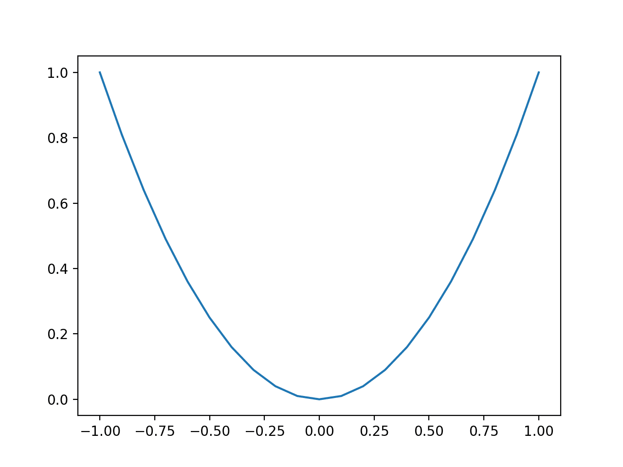
First, let’s define an optimization function.
We will use a simple one-dimensional function that squares the input and defines the range of valid inputs from -1.0 to 1.0.
The objective() function below implements this function.
1
2
3
# objective function
def objective(x):
returnx**2.0
We can then sample all inputs in the range and calculate the objective function value for each.
1
2
3
4
5
6
7
...
# define range for input
r_min,r_max=-1.0,1.0
# sample input range uniformly at 0.1 increments
inputs=arange(r_min,r_max+0.1,0.1)
# compute targets
results=objective(inputs)
Finally, we can create a line plot of the inputs (x-axis) versus the objective function values (y-axis) to get an intuition for the shape of the objective function that we will be searching.
1
2
3
4
5
...
# create a line plot of input vs result
pyplot.plot(inputs,results)
# show the plot
pyplot.show()
The example below ties this together and provides an example of plotting the one-dimensional test function.
1
2
3
4
5
6
7
8
9
10
11
12
13
14
15
16
17
18
# plot of simple function
from numpy import arange
from matplotlib import pyplot
# objective function
def objective(x):
returnx**2.0
# define range for input
r_min,r_max=-1.0,1.0
# sample input range uniformly at 0.1 increments
inputs=arange(r_min,r_max+0.1,0.1)
# compute targets
results=objective(inputs)
# create a line plot of input vs result
pyplot.plot(inputs,results)
# show the plot
pyplot.show()
Running the example creates a line plot of the inputs to the function (x-axis) and the calculated output of the function (y-axis).
We can see the familiar U-shaped called a parabola.
Line Plot of Simple One-Dimensional Function
Next, we can apply the gradient descent algorithm to the problem.
First, we need a function that calculates the derivative for this function.
The derivative of x^2 is x * 2 and the derivative() function implements this below.
1
2
3
# derivative of objective function
def derivative(x):
returnx *2.0
We can then define the bounds of the objective function, the step size, and the number of iterations for the algorithm.
We will use a step size of 0.1 and 30 iterations, both found after a little experimentation.
Running the example starts with a random point in the search space then applies the gradient descent algorithm, reporting performance along the way.
Note: Your results may vary given the stochastic nature of the algorithm or evaluation procedure, or differences in numerical precision. Consider running the example a few times and compare the average outcome.
In this case, we can see that the algorithm finds a good solution after about 20-30 iterations with a function evaluation of about 0.0. Note the optima for this function is at f(0.0) = 0.0.
1
2
3
4
5
6
7
8
9
10
11
12
13
14
15
16
17
18
19
20
21
22
23
24
25
26
27
28
29
30
31
32
>0 f([-0.36308639]) = 0.13183
>1 f([-0.29046911]) = 0.08437
>2 f([-0.23237529]) = 0.05400
>3 f([-0.18590023]) = 0.03456
>4 f([-0.14872018]) = 0.02212
>5 f([-0.11897615]) = 0.01416
>6 f([-0.09518092]) = 0.00906
>7 f([-0.07614473]) = 0.00580
>8 f([-0.06091579]) = 0.00371
>9 f([-0.04873263]) = 0.00237
>10 f([-0.0389861]) = 0.00152
>11 f([-0.03118888]) = 0.00097
>12 f([-0.02495111]) = 0.00062
>13 f([-0.01996089]) = 0.00040
>14 f([-0.01596871]) = 0.00025
>15 f([-0.01277497]) = 0.00016
>16 f([-0.01021997]) = 0.00010
>17 f([-0.00817598]) = 0.00007
>18 f([-0.00654078]) = 0.00004
>19 f([-0.00523263]) = 0.00003
>20 f([-0.0041861]) = 0.00002
>21 f([-0.00334888]) = 0.00001
>22 f([-0.0026791]) = 0.00001
>23 f([-0.00214328]) = 0.00000
>24 f([-0.00171463]) = 0.00000
>25 f([-0.0013717]) = 0.00000
>26 f([-0.00109736]) = 0.00000
>27 f([-0.00087789]) = 0.00000
>28 f([-0.00070231]) = 0.00000
>29 f([-0.00056185]) = 0.00000
Done!
f([-0.00056185]) = 0.000000
Now, let’s get a feeling for the importance of good step size.
Set the step size to a large value, such as 1.0, and re-run the search.
1
2
3
...
# define the step size
step_size=1.0
Run the example with the larger step size and inspect the results.
Note: Your results may vary given the stochastic nature of the algorithm or evaluation procedure, or differences in numerical precision. Consider running the example a few times and compare the average outcome.
We can see that the search does not find the optima, and instead bounces around the domain, in this case between the values 0.64820935 and -0.64820935.
1
2
3
4
5
6
7
8
...
>25 f([0.64820935]) = 0.42018
>26 f([-0.64820935]) = 0.42018
>27 f([0.64820935]) = 0.42018
>28 f([-0.64820935]) = 0.42018
>29 f([0.64820935]) = 0.42018
Done!
f([0.64820935]) = 0.420175
Now, try a much smaller step size, such as 1e-8.
1
2
3
...
# define the step size
step_size=1e-5
Note: Your results may vary given the stochastic nature of the algorithm or evaluation procedure, or differences in numerical precision. Consider running the example a few times and compare the average outcome.
Re-running the search, we can see that the algorithm moves very slowly down the slope of the objective function from the starting point.
1
2
3
4
5
6
7
8
...
>25 f([-0.87315153]) = 0.76239
>26 f([-0.87313407]) = 0.76236
>27 f([-0.8731166]) = 0.76233
>28 f([-0.87309914]) = 0.76230
>29 f([-0.87308168]) = 0.76227
Done!
f([-0.87308168]) = 0.762272
These two quick examples highlight the problems in selecting a step size that is too large or too small and the general importance of testing many different step size values for a given objective function.
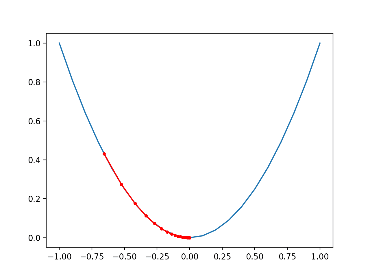
Finally, we can change the learning rate back to 0.1 and visualize the progress of the search on a plot of the target function.
First, we can update the gradient_descent() function to store all solutions and their score found during the optimization as lists and return them at the end of the search instead of the best solution found.
We can create a line plot of the objective function, as before.
1
2
3
4
5
6
7
...
# sample input range uniformly at 0.1 increments
inputs=arange(bounds[0,0],bounds[0,1]+0.1,0.1)
# compute targets
results=objective(inputs)
# create a line plot of input vs result
pyplot.plot(inputs,results)
Finally, we can plot each solution found as a red dot and connect the dots with a line so we can see how the search moved downhill.
1
2
3
...
# plot the solutions found
pyplot.plot(solutions,scores,'.-',color='red')
Tying this all together, the complete example of plotting the result of the gradient descent search on the one-dimensional test function is listed below.
1
2
3
4
5
6
7
8
9
10
11
12
13
14
15
16
17
18
19
20
21
22
23
24
25
26
27
28
29
30
31
32
33
34
35
36
37
38
39
40
41
42
43
44
45
46
47
48
49
50
51
52
53
# example of plotting a gradient descent search on a one-dimensional function
Running the example performs the gradient descent search on the objective function as before, except in this case, each point found during the search is plotted.
Note: Your results may vary given the stochastic nature of the algorithm or evaluation procedure, or differences in numerical precision. Consider running the example a few times and compare the average outcome.
In this case, we can see that the search started about halfway up the left part of the function and stepped downhill to the bottom of the basin.
We can see that in the parts of the objective function with the larger curve, the derivative (gradient) is larger, and in turn, larger steps are taken. Similarly, the gradient is smaller as we get closer to the optima, and in turn, smaller steps are taken.
This highlights that the step size is used as a scale factor on the magnitude of the gradient (curvature) of the objective function.
Plot of the Progress of Gradient Descent on a One Dimensional Objective Function
Further Reading
This section provides more resources on the topic if you are looking to go deeper.
It provides self-study tutorials with full working code on: Gradient Descent, Genetic Algorithms, Hill Climbing, Curve Fitting, RMSProp, Adam,
and much more...
Bring Modern Optimization Algorithms to Your Machine Learning Projects
Thank you Jason. When you have time, could you please write a blog about using pre-trained model for timeseries forecasting/prediction. I saw your post about CNN. I was wondering if you can do a post for pre-trained LSTM or random forest or MLP model
This is a good overview. What I would like to see is a discussion of what to do when you don’t know what the derivative of your target function is. After all, finding the minimum of a parabola is rather trivial. What happens when you have a large, multidimensional space to search and computation time is of the essence? How do you determine the gradient? How do you decide what the step size should be in each dimension? Thank you for this tutorial.
You can use a direct search method (nelder mead) or a stochastic method like a genetic algorithm, simulated annealing, differential evolution, etc if you don’t have a derivative.
Large space means more searching. If eval is slow, you can use a surrogate function/proxy function.
Yes, you can. But the problem is when you have a 2D function, there are infinite number of points (on a circle) around the current point. How to efficiently evaluate the finite difference is the issue. Indeed, Nelder-Mead algorithm is doing just that, see https://machinelearningmastery.com/how-to-use-nelder-mead-optimization-in-python/
You did f(x) = x ^ 2 and f’ is 2x. When x > 0 gradient is positive and you decrease x thereby minimizing loss.
When f(x) = x ^ 2 – 4 though, just adding a constant: gradient also becomes 2x.
Minima will be at x = 2 which is zero. When x = 1, gradient becomes positive and
x := x – alpha * (2x)
will decrease the x instead of increasing it. How do we solve this? (without taking 2nd order derivative)


Good stuff. Your “from scratch” blogs are my favorite!
Thanks!
Thank you Jason. When you have time, could you please write a blog about using pre-trained model for timeseries forecasting/prediction. I saw your post about CNN. I was wondering if you can do a post for pre-trained LSTM or random forest or MLP model
Thanks for the suggestion.
This is a good overview. What I would like to see is a discussion of what to do when you don’t know what the derivative of your target function is. After all, finding the minimum of a parabola is rather trivial. What happens when you have a large, multidimensional space to search and computation time is of the essence? How do you determine the gradient? How do you decide what the step size should be in each dimension? Thank you for this tutorial.
Thanks.
You can use a direct search method (nelder mead) or a stochastic method like a genetic algorithm, simulated annealing, differential evolution, etc if you don’t have a derivative.
Large space means more searching. If eval is slow, you can use a surrogate function/proxy function.
Isn’t it possible to use anyway a gradient descent and estimate the gradient numerically ? using finite difference for instance …
Yes, you can. But the problem is when you have a 2D function, there are infinite number of points (on a circle) around the current point. How to efficiently evaluate the finite difference is the issue. Indeed, Nelder-Mead algorithm is doing just that, see https://machinelearningmastery.com/how-to-use-nelder-mead-optimization-in-python/
Hello Jason,
You did f(x) = x ^ 2 and f’ is 2x. When x > 0 gradient is positive and you decrease x thereby minimizing loss.
When f(x) = x ^ 2 – 4 though, just adding a constant: gradient also becomes 2x.
Minima will be at x = 2 which is zero. When x = 1, gradient becomes positive and
x := x – alpha * (2x)
will decrease the x instead of increasing it. How do we solve this? (without taking 2nd order derivative)
The gradient may be positive or negative, ensuring we move the coefficients in the correct direction to reduce loss.
Oh it’s f = (x-2) ^ 2
not x^2 -4 my bad.
step by step , very clearly for
Thanks!
uhhh where did you find a function named derivative?
You have to define it according to your objective function. For example, if the objective function is f(x)=x*x, then the derivative function is f(x)=x
But if you have a different objective function, returning rmse or roc_auc or some other metric. How do you derive that?
Hi Henrik…the following may be of interest to you:
https://www.statology.org/rmse-python/