
Gradient descent is an optimization algorithm that follows the negative gradient of an objective function in order to locate the minimum of the function.
A limitation of gradient descent is that the progress of the search can slow down if the gradient becomes flat or large curvature. Momentum can be added to gradient descent that incorporates some inertia to updates. This can be further improved by incorporating the gradient of the projected new position rather than the current position, called Nesterov’s Accelerated Gradient (NAG) or Nesterov momentum.
Another limitation of gradient descent is that a single step size (learning rate) is used for all input variables. Extensions to gradient descent like the Adaptive Movement Estimation (Adam) algorithm that uses a separate step size for each input variable but may result in a step size that rapidly decreases to very small values.
Nesterov-accelerated Adaptive Moment Estimation, or the Nadam, is an extension of the Adam algorithm that incorporates Nesterov momentum and can result in better performance of the optimization algorithm.
In this tutorial, you will discover how to develop the gradient descent optimization with Nadam from scratch.
After completing this tutorial, you will know:
- Gradient descent is an optimization algorithm that uses the gradient of the objective function to navigate the search space.
- Nadam is an extension of the Adam version of gradient descent that incorporates Nesterov momentum.
- How to implement the Nadam optimization algorithm from scratch and apply it to an objective function and evaluate the results.
Kick-start your project with my new book Optimization for Machine Learning, including step-by-step tutorials and the Python source code files for all examples.
Let’s get started.
Gradient Descent Optimization With Nadam From Scratch
Photo by BLM Nevada, some rights reserved.
Tutorial Overview
This tutorial is divided into three parts; they are:
- Gradient Descent
- Nadam Optimization Algorithm
- Gradient Descent With Nadam
- Two-Dimensional Test Problem
- Gradient Descent Optimization With Nadam
- Visualization of Nadam Optimization
Gradient Descent
Gradient descent is an optimization algorithm.
It is technically referred to as a first-order optimization algorithm as it explicitly makes use of the first-order derivative of the target objective function.
First-order methods rely on gradient information to help direct the search for a minimum …
— Page 69, Algorithms for Optimization, 2019.
The first-order derivative, or simply the “derivative,” is the rate of change or slope of the target function at a specific point, e.g. for a specific input.
If the target function takes multiple input variables, it is referred to as a multivariate function and the input variables can be thought of as a vector. In turn, the derivative of a multivariate target function may also be taken as a vector and is referred to generally as the gradient.
- Gradient: First-order derivative for a multivariate objective function.
The derivative or the gradient points in the direction of the steepest ascent of the target function for a specific input.
Gradient descent refers to a minimization optimization algorithm that follows the negative of the gradient downhill of the target function to locate the minimum of the function.
The gradient descent algorithm requires a target function that is being optimized and the derivative function for the objective function. The target function f() returns a score for a given set of inputs, and the derivative function f'() gives the derivative of the target function for a given set of inputs.
The gradient descent algorithm requires a starting point (x) in the problem, such as a randomly selected point in the input space.
The derivative is then calculated and a step is taken in the input space that is expected to result in a downhill movement in the target function, assuming we are minimizing the target function.
A downhill movement is made by first calculating how far to move in the input space, calculated as the steps size (called alpha or the learning rate) multiplied by the gradient. This is then subtracted from the current point, ensuring we move against the gradient, or down the target function.
- x(t) = x(t-1) – step_size * f'(x(t))
The steeper the objective function at a given point, the larger the magnitude of the gradient, and in turn, the larger the step taken in the search space. The size of the step taken is scaled using a step size hyperparameter.
- Step Size: Hyperparameter that controls how far to move in the search space against the gradient each iteration of the algorithm.
If the step size is too small, the movement in the search space will be small and the search will take a long time. If the step size is too large, the search may bounce around the search space and skip over the optima.
Now that we are familiar with the gradient descent optimization algorithm, let’s take a look at the Nadam algorithm.
Want to Get Started With Optimization Algorithms?
Take my free 7-day email crash course now (with sample code).
Click to sign-up and also get a free PDF Ebook version of the course.
Nadam Optimization Algorithm
The Nesterov-accelerated Adaptive Moment Estimation, or the Nadam, algorithm is an extension to the Adaptive Movement Estimation (Adam) optimization algorithm to add Nesterov’s Accelerated Gradient (NAG) or Nesterov momentum, which is an improved type of momentum.
More broadly, the Nadam algorithm is an extension to the Gradient Descent Optimization algorithm.
The algorithm was described in the 2016 paper by Timothy Dozat titled “Incorporating Nesterov Momentum into Adam.” Although a version of the paper was written up in 2015 as a Stanford project report with the same name.
Momentum adds an exponentially decaying moving average (first moment) of the gradient to the gradient descent algorithm. This has the impact of smoothing out noisy objective functions and improving convergence.
Adam is an extension of gradient descent that adds a first and second moment of the gradient and automatically adapts a learning rate for each parameter that is being optimized. NAG is an extension to momentum where the update is performed using the gradient of the projected update to the parameter rather than the actual current variable value. This has the effect of slowing down the search when the optima is located rather than overshooting, in some situations.
Nadam is an extension to Adam that uses NAG momentum instead of classical momentum.
We show how to modify Adam’s momentum component to take advantage of insights from NAG, and then we present preliminary evidence suggesting that making this substitution improves the speed of convergence and the quality of the learned models.
— Incorporating Nesterov Momentum into Adam, 2016.
Let’s step through each element of the algorithm.
Nadam uses a decaying step size (alpha) and first moment (mu) hyperparameters that can improve performance. For the case of simplicity, we will ignore this aspect for now and assume constant values.
First, we must maintain the first and second moments of the gradient for each parameter being optimized as part of the search, referred to as m and n respectively. They are initialized to 0.0 at the start of the search.
- m = 0
- n = 0
The algorithm is executed iteratively over time t starting at t=1, and each iteration involves calculating a new set of parameter values x, e.g. going from x(t-1) to x(t).
It is perhaps easy to understand the algorithm if we focus on updating one parameter, which generalizes to updating all parameters via vector operations.
First, the gradient (partial derivatives) are calculated for the current time step.
- g(t) = f'(x(t-1))
Next, the first moment is updated using the gradient and a hyperparameter “mu“.
- m(t) = mu * m(t-1) + (1 – mu) * g(t)
Then the second moment is updated using the “nu” hyperparameter.
- n(t) = nu * n(t-1) + (1 – nu) * g(t)^2
Next, the first moment is bias-corrected using the Nesterov momentum.
- mhat = (mu * m(t) / (1 – mu)) + ((1 – mu) * g(t) / (1 – mu))
The second moment is then bias-corrected.
Note: bias-correction is an aspect of Adam and counters the fact that the first and second moments are initialized to zero at the start of the search.
- nhat = nu * n(t) / (1 – nu)
Finally, we can calculate the value for the parameter for this iteration.
- x(t) = x(t-1) – alpha / (sqrt(nhat) + eps) * mhat
Where alpha is the step size (learning rate) hyperparameter, sqrt() is the square root function, and eps (epsilon) is a small value like 1e-8 added to avoid a divide by zero error.
To review, there are three hyperparameters for the algorithm; they are:
- alpha: Initial step size (learning rate), a typical value is 0.002.
- mu: Decay factor for first moment (beta1 in Adam), a typical value is 0.975.
- nu: Decay factor for second moment (beta2 in Adam), a typical value is 0.999.
And that’s it.
Next, let’s look at how we might implement the algorithm from scratch in Python.
Gradient Descent With Nadam
In this section, we will explore how to implement the gradient descent optimization algorithm with Nadam Momentum.
Two-Dimensional Test Problem
First, let’s define an optimization function.
We will use a simple two-dimensional function that squares the input of each dimension and define the range of valid inputs from -1.0 to 1.0.
The objective() function below implements this function
|
1 2 3 |
# objective function def objective(x, y): return x**2.0 + y**2.0 |
We can create a three-dimensional plot of the dataset to get a feeling for the curvature of the response surface.
The complete example of plotting the objective function is listed below.
|
1 2 3 4 5 6 7 8 9 10 11 12 13 14 15 16 17 18 19 20 21 22 23 24 |
# 3d plot of the test function from numpy import arange from numpy import meshgrid from matplotlib import pyplot # objective function def objective(x, y): return x**2.0 + y**2.0 # define range for input r_min, r_max = -1.0, 1.0 # sample input range uniformly at 0.1 increments xaxis = arange(r_min, r_max, 0.1) yaxis = arange(r_min, r_max, 0.1) # create a mesh from the axis x, y = meshgrid(xaxis, yaxis) # compute targets results = objective(x, y) # create a surface plot with the jet color scheme figure = pyplot.figure() axis = figure.gca(projection='3d') axis.plot_surface(x, y, results, cmap='jet') # show the plot pyplot.show() |
Running the example creates a three-dimensional surface plot of the objective function.
We can see the familiar bowl shape with the global minima at f(0, 0) = 0.
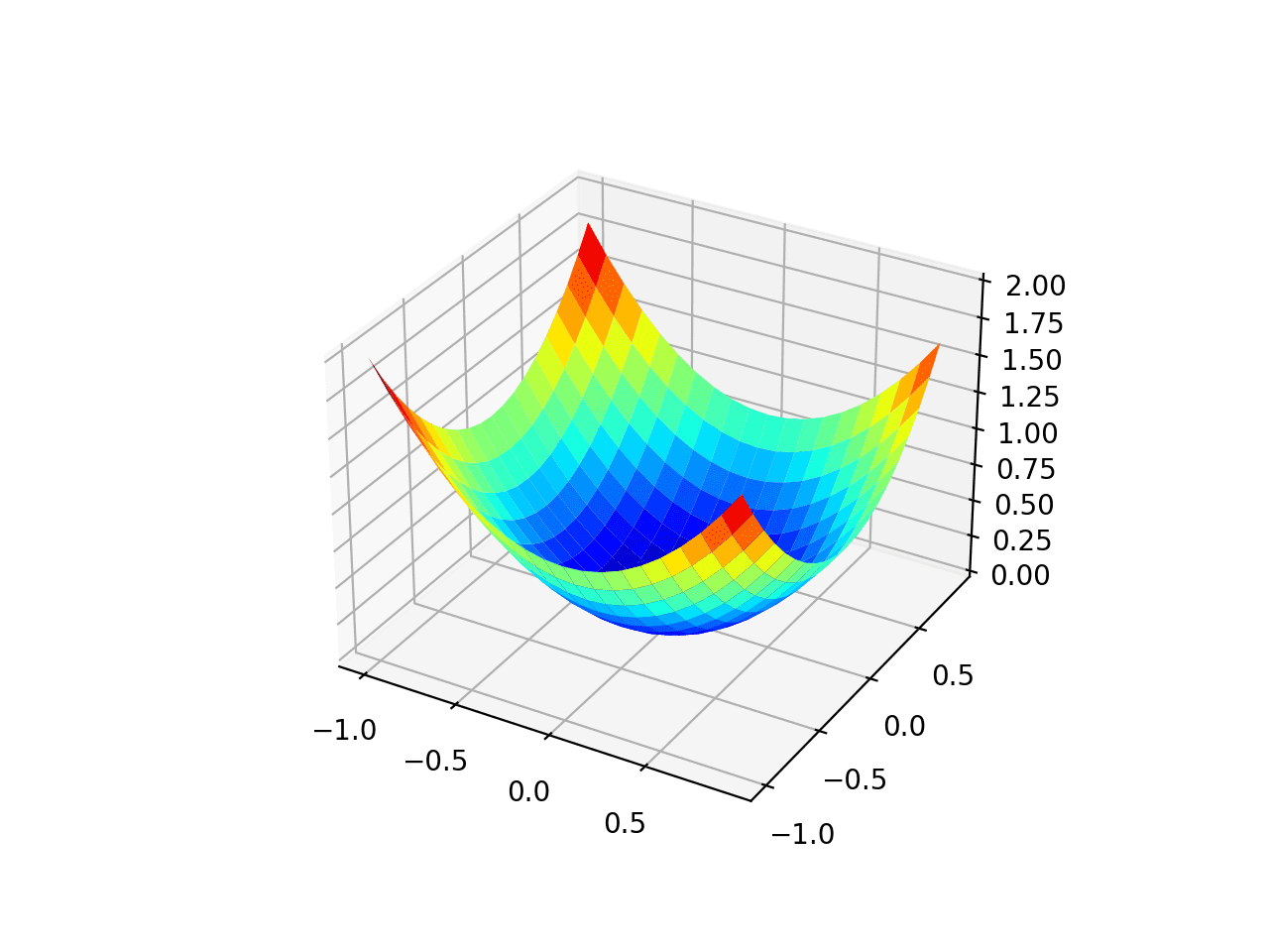
Three-Dimensional Plot of the Test Objective Function
We can also create a two-dimensional plot of the function. This will be helpful later when we want to plot the progress of the search.
The example below creates a contour plot of the objective function.
|
1 2 3 4 5 6 7 8 9 10 11 12 13 14 15 16 17 18 19 20 21 22 23 |
# contour plot of the test function from numpy import asarray from numpy import arange from numpy import meshgrid from matplotlib import pyplot # objective function def objective(x, y): return x**2.0 + y**2.0 # define range for input bounds = asarray([[-1.0, 1.0], [-1.0, 1.0]]) # sample input range uniformly at 0.1 increments xaxis = arange(bounds[0,0], bounds[0,1], 0.1) yaxis = arange(bounds[1,0], bounds[1,1], 0.1) # create a mesh from the axis x, y = meshgrid(xaxis, yaxis) # compute targets results = objective(x, y) # create a filled contour plot with 50 levels and jet color scheme pyplot.contourf(x, y, results, levels=50, cmap='jet') # show the plot pyplot.show() |
Running the example creates a two-dimensional contour plot of the objective function.
We can see the bowl shape compressed to contours shown with a color gradient. We will use this plot to plot the specific points explored during the progress of the search.
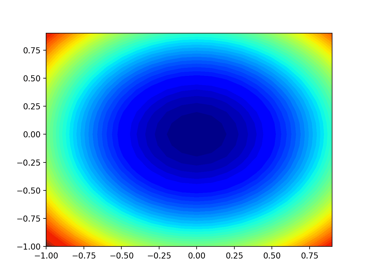
Two-Dimensional Contour Plot of the Test Objective Function
Now that we have a test objective function, let’s look at how we might implement the Nadam optimization algorithm.
Gradient Descent Optimization With Nadam
We can apply the gradient descent with Nadam to the test problem.
First, we need a function that calculates the derivative for this function.
The derivative of x^2 is x * 2 in each dimension.
- f(x) = x^2
- f'(x) = x * 2
The derivative() function implements this below.
|
1 2 3 |
# derivative of objective function def derivative(x, y): return asarray([x * 2.0, y * 2.0]) |
Next, we can implement gradient descent optimization with Nadam.
First, we can select a random point in the bounds of the problem as a starting point for the search.
This assumes we have an array that defines the bounds of the search with one row for each dimension and the first column defines the minimum and the second column defines the maximum of the dimension.
|
1 2 3 4 |
... # generate an initial point x = bounds[:, 0] + rand(len(bounds)) * (bounds[:, 1] - bounds[:, 0]) score = objective(x[0], x[1]) |
Next, we need to initialize the moment vectors.
|
1 2 3 4 |
... # initialize decaying moving averages m = [0.0 for _ in range(bounds.shape[0])] n = [0.0 for _ in range(bounds.shape[0])] |
We then run a fixed number of iterations of the algorithm defined by the “n_iter” hyperparameter.
|
1 2 3 4 |
... # run iterations of gradient descent for t in range(n_iter): ... |
The first step is to calculate the derivative for the current set of parameters.
|
1 2 3 |
... # calculate gradient g(t) g = derivative(x[0], x[1]) |
Next, we need to perform the Nadam update calculations. We will perform these calculations one variable at a time using an imperative programming style for readability.
In practice, I recommend using NumPy vector operations for efficiency.
|
1 2 3 4 |
... # build a solution one variable at a time for i in range(x.shape[0]): ... |
First, we need to calculate the moment vector.
|
1 2 3 |
... # m(t) = mu * m(t-1) + (1 - mu) * g(t) m[i] = mu * m[i] + (1.0 - mu) * g[i] |
Then the second moment vector.
|
1 2 3 |
... # n(t) = nu * n(t-1) + (1 - nu) * g(t)^2 n[i] = nu * n[i] + (1.0 - nu) * g[i]**2 |
Then the bias-corrected Nesterov momentum.
|
1 2 3 |
... # mhat = (mu * m(t) / (1 - mu)) + ((1 - mu) * g(t) / (1 - mu)) mhat = (mu * m[i] / (1.0 - mu)) + ((1 - mu) * g[i] / (1.0 - mu)) |
The bias-correct second moment.
|
1 2 3 |
... # nhat = nu * n(t) / (1 - nu) nhat = nu * n[i] / (1.0 - nu) |
And finally updating the parameter.
|
1 2 3 |
... # x(t) = x(t-1) - alpha / (sqrt(nhat) + eps) * mhat x[i] = x[i] - alpha / (sqrt(nhat) + eps) * mhat |
This is then repeated for each parameter that is being optimized.
At the end of the iteration, we can evaluate the new parameter values and report the performance of the search.
|
1 2 3 4 5 |
... # evaluate candidate point score = objective(x[0], x[1]) # report progress print('>%d f(%s) = %.5f' % (t, x, score)) |
We can tie all of this together into a function named nadam() that takes the names of the objective and derivative functions, as well as the algorithm hyperparameters, and returns the best solution found at the end of the search and its evaluation.
|
1 2 3 4 5 6 7 8 9 10 11 12 13 14 15 16 17 18 19 20 21 22 23 24 25 26 27 28 29 |
# gradient descent algorithm with nadam def nadam(objective, derivative, bounds, n_iter, alpha, mu, nu, eps=1e-8): # generate an initial point x = bounds[:, 0] + rand(len(bounds)) * (bounds[:, 1] - bounds[:, 0]) score = objective(x[0], x[1]) # initialize decaying moving averages m = [0.0 for _ in range(bounds.shape[0])] n = [0.0 for _ in range(bounds.shape[0])] # run the gradient descent for t in range(n_iter): # calculate gradient g(t) g = derivative(x[0], x[1]) # build a solution one variable at a time for i in range(bounds.shape[0]): # m(t) = mu * m(t-1) + (1 - mu) * g(t) m[i] = mu * m[i] + (1.0 - mu) * g[i] # n(t) = nu * n(t-1) + (1 - nu) * g(t)^2 n[i] = nu * n[i] + (1.0 - nu) * g[i]**2 # mhat = (mu * m(t) / (1 - mu)) + ((1 - mu) * g(t) / (1 - mu)) mhat = (mu * m[i] / (1.0 - mu)) + ((1 - mu) * g[i] / (1.0 - mu)) # nhat = nu * n(t) / (1 - nu) nhat = nu * n[i] / (1.0 - nu) # x(t) = x(t-1) - alpha / (sqrt(nhat) + eps) * mhat x[i] = x[i] - alpha / (sqrt(nhat) + eps) * mhat # evaluate candidate point score = objective(x[0], x[1]) # report progress print('>%d f(%s) = %.5f' % (t, x, score)) return [x, score] |
We can then define the bounds of the function and the hyperparameters and call the function to perform the optimization.
In this case, we will run the algorithm for 50 iterations with an initial alpha of 0.02, mu of 0.8 and a nu of 0.999, found after a little trial and error.
|
1 2 3 4 5 6 7 8 9 10 11 12 13 14 15 |
... # seed the pseudo random number generator seed(1) # define range for input bounds = asarray([[-1.0, 1.0], [-1.0, 1.0]]) # define the total iterations n_iter = 50 # steps size alpha = 0.02 # factor for average gradient mu = 0.8 # factor for average squared gradient nu = 0.999 # perform the gradient descent search with nadam best, score = nadam(objective, derivative, bounds, n_iter, alpha, mu, nu) |
At the end of the run, we will report the best solution found.
|
1 2 3 4 |
... # summarize the result print('Done!') print('f(%s) = %f' % (best, score)) |
Tying all of this together, the complete example of Nadam gradient descent applied to our test problem is listed below.
|
1 2 3 4 5 6 7 8 9 10 11 12 13 14 15 16 17 18 19 20 21 22 23 24 25 26 27 28 29 30 31 32 33 34 35 36 37 38 39 40 41 42 43 44 45 46 47 48 49 50 51 52 53 54 55 56 57 58 59 60 |
# gradient descent optimization with nadam for a two-dimensional test function from math import sqrt from numpy import asarray from numpy.random import rand from numpy.random import seed # objective function def objective(x, y): return x**2.0 + y**2.0 # derivative of objective function def derivative(x, y): return asarray([x * 2.0, y * 2.0]) # gradient descent algorithm with nadam def nadam(objective, derivative, bounds, n_iter, alpha, mu, nu, eps=1e-8): # generate an initial point x = bounds[:, 0] + rand(len(bounds)) * (bounds[:, 1] - bounds[:, 0]) score = objective(x[0], x[1]) # initialize decaying moving averages m = [0.0 for _ in range(bounds.shape[0])] n = [0.0 for _ in range(bounds.shape[0])] # run the gradient descent for t in range(n_iter): # calculate gradient g(t) g = derivative(x[0], x[1]) # build a solution one variable at a time for i in range(bounds.shape[0]): # m(t) = mu * m(t-1) + (1 - mu) * g(t) m[i] = mu * m[i] + (1.0 - mu) * g[i] # n(t) = nu * n(t-1) + (1 - nu) * g(t)^2 n[i] = nu * n[i] + (1.0 - nu) * g[i]**2 # mhat = (mu * m(t) / (1 - mu)) + ((1 - mu) * g(t) / (1 - mu)) mhat = (mu * m[i] / (1.0 - mu)) + ((1 - mu) * g[i] / (1.0 - mu)) # nhat = nu * n(t) / (1 - nu) nhat = nu * n[i] / (1.0 - nu) # x(t) = x(t-1) - alpha / (sqrt(nhat) + eps) * mhat x[i] = x[i] - alpha / (sqrt(nhat) + eps) * mhat # evaluate candidate point score = objective(x[0], x[1]) # report progress print('>%d f(%s) = %.5f' % (t, x, score)) return [x, score] # seed the pseudo random number generator seed(1) # define range for input bounds = asarray([[-1.0, 1.0], [-1.0, 1.0]]) # define the total iterations n_iter = 50 # steps size alpha = 0.02 # factor for average gradient mu = 0.8 # factor for average squared gradient nu = 0.999 # perform the gradient descent search with nadam best, score = nadam(objective, derivative, bounds, n_iter, alpha, mu, nu) print('Done!') print('f(%s) = %f' % (best, score)) |
Running the example applies the optimization algorithm with Nadam to our test problem and reports the performance of the search for each iteration of the algorithm.
Note: Your results may vary given the stochastic nature of the algorithm or evaluation procedure, or differences in numerical precision. Consider running the example a few times and compare the average outcome.
In this case, we can see that a near-optimal solution was found after perhaps 44 iterations of the search, with input values near 0.0 and 0.0, evaluating to 0.0.
|
1 2 3 4 5 6 7 8 9 10 11 12 13 |
... >40 f([ 5.07445337e-05 -3.32910019e-03]) = 0.00001 >41 f([-1.84325171e-05 -3.00939427e-03]) = 0.00001 >42 f([-6.78814472e-05 -2.69839367e-03]) = 0.00001 >43 f([-9.88339249e-05 -2.40042096e-03]) = 0.00001 >44 f([-0.00011368 -0.00211861]) = 0.00000 >45 f([-0.00011547 -0.00185511]) = 0.00000 >46 f([-0.0001075 -0.00161122]) = 0.00000 >47 f([-9.29922627e-05 -1.38760991e-03]) = 0.00000 >48 f([-7.48258406e-05 -1.18436586e-03]) = 0.00000 >49 f([-5.54299505e-05 -1.00116899e-03]) = 0.00000 Done! f([-5.54299505e-05 -1.00116899e-03]) = 0.000001 |
Visualization of Nadam Optimization
We can plot the progress of the Nadam search on a contour plot of the domain.
This can provide an intuition for the progress of the search over the iterations of the algorithm.
We must update the nadam() function to maintain a list of all solutions found during the search, then return this list at the end of the search.
The updated version of the function with these changes is listed below.
|
1 2 3 4 5 6 7 8 9 10 11 12 13 14 15 16 17 18 19 20 21 22 23 24 25 26 27 28 29 30 31 32 |
# gradient descent algorithm with nadam def nadam(objective, derivative, bounds, n_iter, alpha, mu, nu, eps=1e-8): solutions = list() # generate an initial point x = bounds[:, 0] + rand(len(bounds)) * (bounds[:, 1] - bounds[:, 0]) score = objective(x[0], x[1]) # initialize decaying moving averages m = [0.0 for _ in range(bounds.shape[0])] n = [0.0 for _ in range(bounds.shape[0])] # run the gradient descent for t in range(n_iter): # calculate gradient g(t) g = derivative(x[0], x[1]) # build a solution one variable at a time for i in range(bounds.shape[0]): # m(t) = mu * m(t-1) + (1 - mu) * g(t) m[i] = mu * m[i] + (1.0 - mu) * g[i] # n(t) = nu * n(t-1) + (1 - nu) * g(t)^2 n[i] = nu * n[i] + (1.0 - nu) * g[i]**2 # mhat = (mu * m(t) / (1 - mu)) + ((1 - mu) * g(t) / (1 - mu)) mhat = (mu * m[i] / (1.0 - mu)) + ((1 - mu) * g[i] / (1.0 - mu)) # nhat = nu * n(t) / (1 - nu) nhat = nu * n[i] / (1.0 - nu) # x(t) = x(t-1) - alpha / (sqrt(nhat) + eps) * mhat x[i] = x[i] - alpha / (sqrt(nhat) + eps) * mhat # evaluate candidate point score = objective(x[0], x[1]) # store solution solutions.append(x.copy()) # report progress print('>%d f(%s) = %.5f' % (t, x, score)) return solutions |
We can then execute the search as before, and this time retrieve the list of solutions instead of the best final solution.
|
1 2 3 4 5 6 7 8 9 10 11 12 13 14 15 |
... # seed the pseudo random number generator seed(1) # define range for input bounds = asarray([[-1.0, 1.0], [-1.0, 1.0]]) # define the total iterations n_iter = 50 # steps size alpha = 0.02 # factor for average gradient mu = 0.8 # factor for average squared gradient nu = 0.999 # perform the gradient descent search with nadam solutions = nadam(objective, derivative, bounds, n_iter, alpha, mu, nu) |
We can then create a contour plot of the objective function, as before.
|
1 2 3 4 5 6 7 8 9 10 |
... # sample input range uniformly at 0.1 increments xaxis = arange(bounds[0,0], bounds[0,1], 0.1) yaxis = arange(bounds[1,0], bounds[1,1], 0.1) # create a mesh from the axis x, y = meshgrid(xaxis, yaxis) # compute targets results = objective(x, y) # create a filled contour plot with 50 levels and jet color scheme pyplot.contourf(x, y, results, levels=50, cmap='jet') |
Finally, we can plot each solution found during the search as a white dot connected by a line.
|
1 2 3 4 |
... # plot the sample as black circles solutions = asarray(solutions) pyplot.plot(solutions[:, 0], solutions[:, 1], '.-', color='w') |
Tying this all together, the complete example of performing the Nadam optimization on the test problem and plotting the results on a contour plot is listed below.
|
1 2 3 4 5 6 7 8 9 10 11 12 13 14 15 16 17 18 19 20 21 22 23 24 25 26 27 28 29 30 31 32 33 34 35 36 37 38 39 40 41 42 43 44 45 46 47 48 49 50 51 52 53 54 55 56 57 58 59 60 61 62 63 64 65 66 67 68 69 70 71 72 73 74 75 76 77 78 79 80 |
# example of plotting the nadam search on a contour plot of the test function from math import sqrt from numpy import asarray from numpy import arange from numpy import product from numpy.random import rand from numpy.random import seed from numpy import meshgrid from matplotlib import pyplot from mpl_toolkits.mplot3d import Axes3D # objective function def objective(x, y): return x**2.0 + y**2.0 # derivative of objective function def derivative(x, y): return asarray([x * 2.0, y * 2.0]) # gradient descent algorithm with nadam def nadam(objective, derivative, bounds, n_iter, alpha, mu, nu, eps=1e-8): solutions = list() # generate an initial point x = bounds[:, 0] + rand(len(bounds)) * (bounds[:, 1] - bounds[:, 0]) score = objective(x[0], x[1]) # initialize decaying moving averages m = [0.0 for _ in range(bounds.shape[0])] n = [0.0 for _ in range(bounds.shape[0])] # run the gradient descent for t in range(n_iter): # calculate gradient g(t) g = derivative(x[0], x[1]) # build a solution one variable at a time for i in range(bounds.shape[0]): # m(t) = mu * m(t-1) + (1 - mu) * g(t) m[i] = mu * m[i] + (1.0 - mu) * g[i] # n(t) = nu * n(t-1) + (1 - nu) * g(t)^2 n[i] = nu * n[i] + (1.0 - nu) * g[i]**2 # mhat = (mu * m(t) / (1 - mu)) + ((1 - mu) * g(t) / (1 - mu)) mhat = (mu * m[i] / (1.0 - mu)) + ((1 - mu) * g[i] / (1.0 - mu)) # nhat = nu * n(t) / (1 - nu) nhat = nu * n[i] / (1.0 - nu) # x(t) = x(t-1) - alpha / (sqrt(nhat) + eps) * mhat x[i] = x[i] - alpha / (sqrt(nhat) + eps) * mhat # evaluate candidate point score = objective(x[0], x[1]) # store solution solutions.append(x.copy()) # report progress print('>%d f(%s) = %.5f' % (t, x, score)) return solutions # seed the pseudo random number generator seed(1) # define range for input bounds = asarray([[-1.0, 1.0], [-1.0, 1.0]]) # define the total iterations n_iter = 50 # steps size alpha = 0.02 # factor for average gradient mu = 0.8 # factor for average squared gradient nu = 0.999 # perform the gradient descent search with nadam solutions = nadam(objective, derivative, bounds, n_iter, alpha, mu, nu) # sample input range uniformly at 0.1 increments xaxis = arange(bounds[0,0], bounds[0,1], 0.1) yaxis = arange(bounds[1,0], bounds[1,1], 0.1) # create a mesh from the axis x, y = meshgrid(xaxis, yaxis) # compute targets results = objective(x, y) # create a filled contour plot with 50 levels and jet color scheme pyplot.contourf(x, y, results, levels=50, cmap='jet') # plot the sample as black circles solutions = asarray(solutions) pyplot.plot(solutions[:, 0], solutions[:, 1], '.-', color='w') # show the plot pyplot.show() |
Running the example performs the search as before, except in this case, the contour plot of the objective function is created.
In this case, we can see that a white dot is shown for each solution found during the search, starting above the optima and progressively getting closer to the optima at the center of the plot.
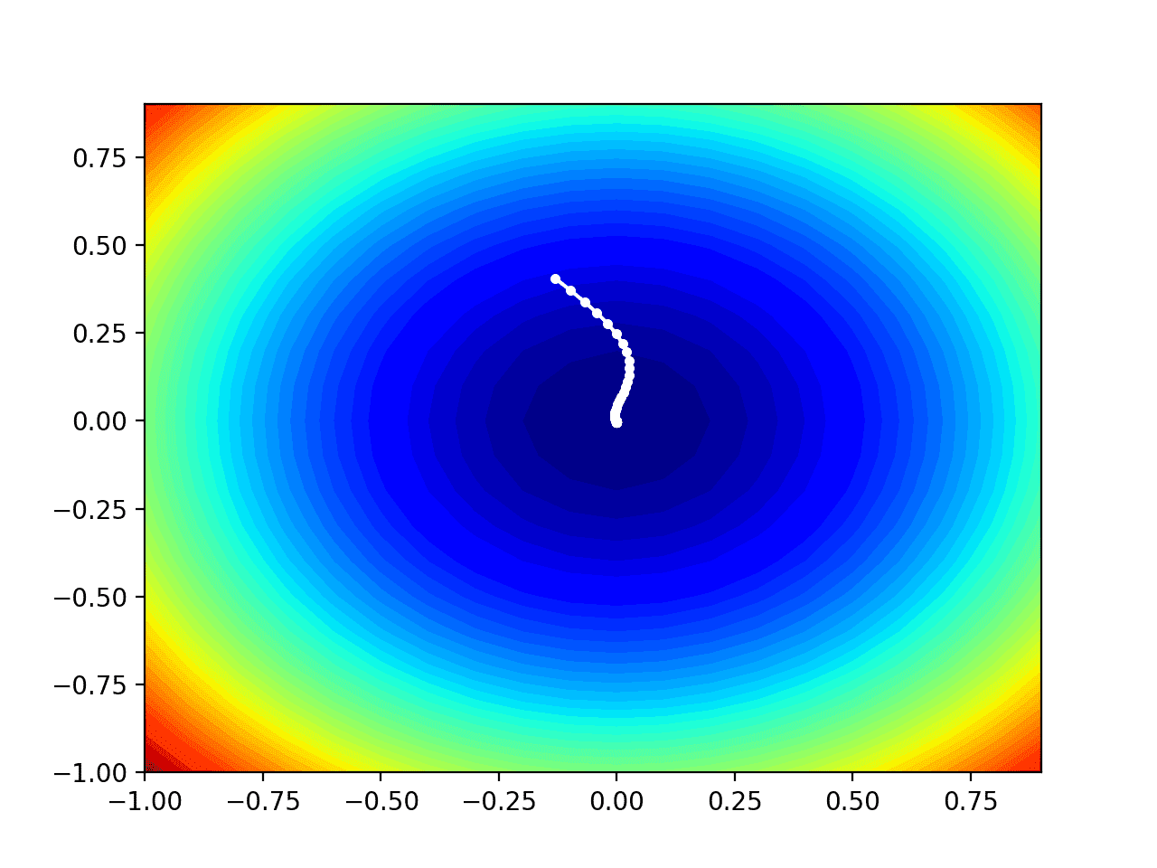
Contour Plot of the Test Objective Function With Nadam Search Results Shown
Further Reading
This section provides more resources on the topic if you are looking to go deeper.
Papers
- Incorporating Nesterov Momentum into Adam, 2016.
- Incorporating Nesterov Momentum into Adam, Stanford Report, 2015.
- A method for solving the convex programming problem with convergence rate O (1/k^2), 1983.
- Adam: A Method for Stochastic Optimization, 2014.
- An Overview Of Gradient Descent Optimization Algorithms, 2016.
Books
- Algorithms for Optimization, 2019.
- Deep Learning, 2016.
APIs
Articles
- Gradient descent, Wikipedia.
- Stochastic gradient descent, Wikipedia.
- Optimization, Timothy Dozat, GitHub.
Summary
In this tutorial, you discovered how to develop the gradient descent optimization with Nadam from scratch.
Specifically, you learned:
- Gradient descent is an optimization algorithm that uses the gradient of the objective function to navigate the search space.
- Nadam is an extension of the Adam version of gradient descent that incorporates Nesterov momentum.
- How to implement the Nadam optimization algorithm from scratch and apply it to an objective function and evaluate the results.
Do you have any questions?
Ask your questions in the comments below and I will do my best to answer.
Get a Handle on Modern Optimization Algorithms!

Develop Your Understanding of Optimization
...with just a few lines of python code
Discover how in my new Ebook:
Optimization for Machine Learning
It provides self-study tutorials with full working code on:
Gradient Descent, Genetic Algorithms, Hill Climbing, Curve Fitting, RMSProp, Adam,
and much more...


Thank you for another great tutorial Jason. Very well explained and demonstrated.
You’re welcome!
Hi, Jason, great article!
But I’m confused about this part in code:
mhat = (mu * m[i] / (1.0 – mu)) + ( (1 – mu) * g[i] / (1.0 – mu) )
I guess (1 – mu) * g[i] / (1.0 – mu) contains a typo, since it’s equal to g[i].
Thanks!
Excellent question!
Yes, it’s correct – but simplified.
Typically in the final piece “mu” is calculated as a decaying values, e.g. mu(t). You can see this in the Nadam paper, and in Ruder’s summary paper.
Dear Dr Jason,
First thank you for another ‘from scratch’ demonstration of optimization with ‘NADAM’ and the previous ‘from scratch’ involving “Nesterov Momentum” at https://machinelearningmastery.com/gradient-descent-with-nesterov-momentum-from-scratch/
Yes there is a NADAM implementation at https://www.tensorflow.org/api_docs/python/tf/keras/optimizers/Nadam and the ‘from scratch’ series of algorithms are “under the hood” versions for learning how these algorithms.
QUESTION PLEASE:
Does the NADAM which is an implementation of “Nesterov Momentum” of RMSProp offer any advatage(s) over the “Nesterov Momentum” or “Adam” optimizers OR do you use all the algorithms to find out which gives the most optimum results?
Thank you in advance
Anthony of Sydney
It can help on some problems.
You can trial different optimizers, or if you have some idea about the objective function or familiarity with a given optimizer you may want to choose one over another.
Dear Dr Jason,
Thank you,
Anthony of Sydney
You’re welcome.