Training and Validation Data in PyTorch

Training data is the set of data that a machine learning algorithm uses to learn. It is also called training set. Validation data is one of the sets of data that machine learning algorithms use to test their accuracy. To validate an algorithm’s performance is to compare its predicted output with the known ground truth in validation data.

Training data is usually large and complex, while validation data is usually smaller. The more training examples there are, the better the model performance will be. For instance, in a spam detection task, if there are 10 spam emails and 10 non-spam emails in the training set then it can be difficult for the machine learning model to detect spam in a new email because there isn’t enough information about what spam looks like. However, if we have 10 million spam emails and 10 million non-spam emails then it would be much easier for our model to detect new spam because it has seen so many examples of what it looks like.

In this tutorial, you will learn about training and validation data in PyTorch. We will also demonstrate the importance of training and validation data for machine learning models in general, with a focus on neural networks. Particularly, you’ll learn:

• The concept of training and validation data in PyTorch.
• How data is split into training and validations sets in PyTorch.
• How you can build a simple linear regression model with built-in functions in PyTorch.
• How you can use various learning rates to train our model in order to get the desired accuracy.
• How you can tune the hyperparameters in order to obtain the best model for your data.

Kick-start your project with my book Deep Learning with PyTorch. It provides self-study tutorials with working code.

Using Optimizers from PyTorch.
Picture by Markus Krisetya. Some rights reserved.

Overview

This tutorial is in three parts; they are

• Build the Data Class for Training and Validation Sets
• Build and Train the Model
• Visualize the Results

Build the Data Class for Training and Validation Sets

Let’s first load up a few libraries we’ll need in this tutorial.

We’ll start from building a custom dataset class to produce enough amount of synthetic data. This will allow us to split our data into training set and validation set. Moreover, we’ll add some steps to include the outliers into the data as well.

For training set, we’ll set our train parameter to True by default. If set to False, it will produce validation data. We created our train set and validation set as separate objects.

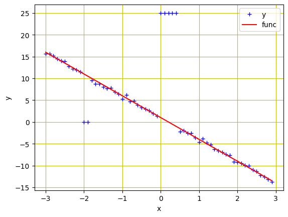
Now, let’s visualize our data. You’ll see the outliers at $x=-2$ and $x=0$.

Training and validation datasets

The complete code to generate the plot above is as follows.

Build and Train the Model

The nn package in PyTorch provides us many useful functions. We’ll import linear regression model and loss criterion from the nn package. Furthermore, we’ll also import DataLoader from torch.utils.data package.

We’ll create a list of various learning rates to train multiple models in one go. This is a common practice among deep learning practitioners where they tune different hyperparameters to get the best model. We’ll store both training and validation losses in tensors and create an empty list Models to store our models as well. Later on, we’ll plot the graphs to evaluate our models.

To train the models, we’ll use various learning rates with stochastic gradient descent (SGD) optimizer. Results for training and validation data will be saved along with the models in the list. We’ll train all models for 20 epochs.

The code above collects losses from training and validation separately. This helps us to understand how well our training can be, for example, whether we are overfitting. It overfits if we discovered that the loss in validation set is largely different from the loss from training set. In that case, our trained model failed to generalize to the data it didn’t see, namely, the validation sets.

Visualize the Results

In the above, we use the same model (linear regression) and train with a fixed number of epochs. The only variation is the learning rate. Then we can compare which learning rate gives us the best model in terms of fastest convergence.

Let’s visualize the loss plots for both training and validation data for each learning rate. By looking at the plot, you can observe that the loss is smallest at the learning rate 0.001, meaning our model converge faster at this learning rate for this data.

Loss vs learning rate

Let’s also plot the predictions from each of the models on the validation data. A perfectly converged model should fit the data perfectly while a model far from converged would produce predicts that are far off from the data.

which we see the prediction visualized as follows:

As you can see, the green line is closer to the validation data points. It’s the line with the optimal learning rate (0.001).

The following is the complete code from creating the data to visualizing the loss from training and validation.

Summary

In this tutorial, you learned the concept of training and validation data in PyTorch. Particularly, you learned:

• The concept of training and validation data in PyTorch.
• How data is split into training and validations sets in PyTorch.
• How you can build a simple linear regression model with built-in functions in PyTorch.
• How you can use various learning rates to train our model in order to get the desired accuracy.
• How you can tune the hyperparameters in order to obtain the best model for your data.

Get Started on Deep Learning with PyTorch!

Learn how to build deep learning models

...using the newly released PyTorch 2.0 library

Discover how in my new Ebook:
Deep Learning with PyTorch

It provides self-study tutorials with hundreds of working code to turn you from a novice to expert. It equips you with
tensor operation, training, evaluation, hyperparameter optimization, and much more...

Kick-start your deep learning journey with hands-on exercises

See What's Inside