The traditional model of neural network is called multilayer perceptrons. They are usually made up of a series of interconnected layers. The input layer is where the data enters the network, and the output layer is where the network delivers the output.
The input layer is usually connected to one or more hidden layers, which modify and process the data before it reaches the output layer. The hidden layers are what make neural networks so powerful: they can learn complicated functions that might be difficult for a programmer to specify in code.
In the previous tutorial, we built a neural network with only a couple of hidden neurons. Here, you will implement a neural network by adding more hidden neurons to it. This will estimate more complex function for us in order to fit the data.
During the implementation process, you’ll learn:
- How to build a neural network with more hidden neurons in PyTorch.
- How to estimate complex functions using neural networks by adding more hidden neurons to the network.
- How to train a neural network in PyTorch.
Kick-start your project with my book Deep Learning with PyTorch. It provides self-study tutorials with working code.
Let’s get started.

Neural Network with More Hidden Neurons.
Picture by Kdwk Leung. Some rights reserved.
Overview
This tutorial is in three parts; they are
- Preparing the Data
- Build the Model Architecture
- Train the Model
Preparing the Data
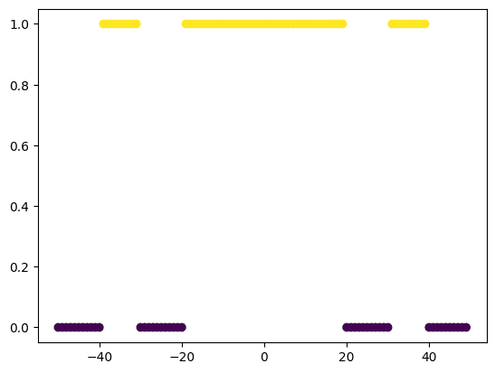
Let’s build a Data class that extends the Dataset class from PyTorch. You use it to create a dataset of 100 synthetic values ranging from $-50$ to $50$. The x tensor stores the values in the specified range, while the y tensor is a corresponding tensor of zeros with the same shape as x.
Next, you use a for loop to set the values in x and y tensors based on the values in x. If a value in x is between $-20$ and $20$, the corresponding value in y is set to 1 and if a value in x is between $-30$ and $-20$ or between $20$ and $30$, the corresponding value in y is set to 0. Similarly, If a value in x is between $-40$ and $-30$ or between $30$ and $40$, the corresponding value in y is set to 1. Otherwise, the corresponding value in y is set to 0.
In the Data class, the __getitem__() method has been used to retrieve the x and y values at a specified index in the dataset. The __len__() method returns the length of the dataset. With these, you can obtain a sample from the dataset using data[i] and tell the size of the dataset using len(data). This class can be used to create a data object that can be passed to a PyTorch data loader to train a machine learning model.
Note that you are building this complex data object to see how well our neural network with more hidden neurons estimates the function. Here is how the code of the data object will look like.
|
1 2 3 4 5 6 7 8 9 10 11 12 13 14 15 16 17 18 19 20 21 22 23 24 25 26 27 28 29 30 31 32 33 |
import torch from torch.utils.data import Dataset, DataLoader class Data(Dataset): def __init__(self): # Create tensor of 100 values from -50 to 50 self.x = torch.zeros(100, 1) # Create tensor of zeros with the same shape as x self.y = torch.zeros(self.x.shape) # Set the values in x and y using a for loop for i in range(100): self.x[i] = -50 + i if self.x[i,0] > -20 and self.x[i,0] < 20: self.y[i] = 1 elif (self.x[i,0] > -30 and self.x[i,0] < -20) or (self.x[i,0] > 20 and self.x[i,0] < 30): self.y[i] = 0 elif (self.x[i,0] > -40 and self.x[i,0] < -30) or (self.x[i,0] > 30 and self.x[i,0] < 40): self.y[i] = 1 else: self.y[i] = 0 # Store the length of the dataset self.len = self.x.shape[0] def __getitem__(self, index): # Return the x and y values at the specified index return self.x[index], self.y[index] def __len__(self): # Return the length of the dataset return self.len |
Let’s instantiate a data object.
|
1 2 |
# Create the Data object dataset = Data() |
And, write a function to visualize this data, which will also be useful when you train the model later.
|
1 2 3 4 5 6 7 8 9 10 11 12 13 14 15 16 17 18 19 20 |
import pandas as pd import matplotlib.pyplot as plt def plot_data(X, Y, model=None, leg=False): # Get the x and y values from the Data object x = dataset.x y = dataset.y # Convert the x and y values to a Pandas series with an index x = pd.Series(x[:, 0], index=range(len(x))) y = pd.Series(y[:, 0], index=range(len(y))) # Scatter plot of the x and y values, coloring the points by their labels plt.scatter(x, y, c=y) if model!=None: plt.plot(X.numpy(), model(X).detach().numpy(), label='Neural Net') # Show the plot plt.show() |
If you run this function, you can see the data looks like the following:
|
1 |
plot_data(dataset.x, dataset.y, leg=False) |
Want to Get Started With Deep Learning with PyTorch?
Take my free email crash course now (with sample code).
Click to sign-up and also get a free PDF Ebook version of the course.
Build the Model Architecture
Below, you will define a NeuralNetwork class to build a custom model architecture using nn.Module from PyTorch. This class represents a simple neural network with an input layer, a hidden layer, and an output layer.
The __init__() method is used to initialize the neural network by defining the layers in the network. The forward method is used to define the forward pass through the network. In this case, a sigmoid activation function is applied to the output of both input and output layers. This means that the output of the network will be a value between 0 and 1.
Finally, you will create an instance of the NeuralNetwork class and store it in the model variable. The model is initialized with an input layer having 1 input neuron, a hidden layer having 15 hidden neurons, and an output layer having 1 output neuron. This model is now ready to be trained on some data.
|
1 2 3 4 5 6 7 8 9 10 11 12 13 14 15 16 17 18 |
import torch.nn as nn # Define the Neural Network class NeuralNetwork(nn.Module): def __init__(self, input_size, hidden_size, output_size): super().__init__() # Define the layers in the neural network self.input_layer = nn.Linear(input_size, hidden_size) self.output_layer = nn.Linear(hidden_size, output_size) def forward(self, x): # Define the forward pass through the network x = torch.sigmoid(self.input_layer(x)) x = torch.sigmoid(self.output_layer(x)) return x # Initialize the Neural Network model = NeuralNetwork(input_size=1, hidden_size=20, output_size=1) |
Train the Model
Let’s define the criterion, optimizer, and dataloader. You should use binary cross entropy loss as the dataset is a classification with two classes. Adam optimizer is used, with a batch size of 32. The learning rate is set to 0.01 which determines how model weights are updated during training. The loss function is used to evaluate the model performance, the optimizer updates the weights, and the data loader divides the data into batches for efficient processing.
|
1 2 3 4 |
learning_rate = 0.01 criterion = nn.BCELoss() optimizer = torch.optim.Adam(model.parameters(), lr=learning_rate) data_loader = DataLoader(dataset=dataset, batch_size=32) |
Now, let’s build a training loop for 7000 epochs and visualize the results during training. You’ll see how well our model estimates the data points as the training progresses.
|
1 2 3 4 5 6 7 8 9 10 11 12 13 14 15 16 17 18 19 20 21 22 23 24 25 26 27 28 |
n_epochs = 7000 # number of epochs to train the model LOSS = [] # list to store the loss values after each epoch # train the model for n_epochs for epoch in range(n_epochs): total = 0 # variable to store the total loss for this epoch # iterate over the data in the data loader for x, y in data_loader: # zero the gradients of the model optimizer.zero_grad() # make a prediction using the model yhat = model(x) # compute the loss between the predicted and true values loss = criterion(yhat, y) # compute the gradients of the model with respect to the loss loss.backward() # update the model parameters optimizer.step() # add the loss value to the total loss for this epoch total += loss.item() # after each epoch, check if the epoch number is divisible by 200 if epoch % 1000 == 0: # if it is, plot the current data and model using the PlotData function plot_data(dataset.x, dataset.y, model) # print the current loss print(f"Epochs Done: {epoch+1}/{n_epochs}, Loss: {loss.item():.4f}") # add the total loss for this epoch to the LOSS list LOSS.append(total) |
When you run this loop, you will see at the first epoch, the neural network modelled the dataset poorly, like the following: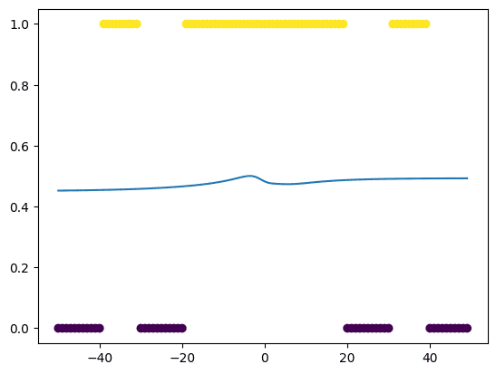
But the accuracy improved as the training progressed. After the training loop completed, we can see the result as the neural network modelled the data like the following:
|
1 2 |
# plot after training loop ended plot_data(dataset.x, dataset.y, model) |

and the corresponding history of loss metric can be plot like the following:
|
1 2 3 4 5 6 7 |
# create a plot of the loss over epochs plt.figure() plt.plot(LOSS) plt.xlabel('epochs') plt.ylabel('loss') # show the plot plt.show() |
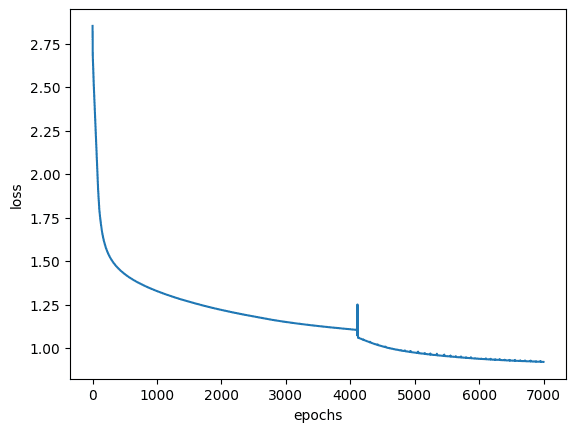
As you can see, our model estimated the function quite well but not perfect. The input of range 20 to 40, for example, isn’t predicted right. You may try to expand the network to add one more layer, such as the following, and see if it will make any difference.
|
1 2 3 4 5 6 7 8 9 10 11 12 13 14 15 16 17 18 19 |
# Define the Neural Network class NeuralNetwork(nn.Module): def __init__(self, input_size, hidden1_size, hidden2_size, output_size): super(NeuralNetwork, self).__init__() # Define the layers in the neural network self.layer1 = nn.Linear(input_size, hidden1_size) self.layer2 = nn.Linear(hidden1_size, hidden2_size) self.output_layer = nn.Linear(hidden2_size, output_size) def forward(self, x): # Define the forward pass through the network x = torch.sigmoid(self.layer1(x)) x = torch.sigmoid(self.layer2(x)) x = torch.sigmoid(self.output_layer(x)) return x # Initialize the Neural Network model = NeuralNetwork(input_size=1, hidden1_size=10, hidden2_size=10, output_size=1) |
Putting everything together, the following is the complete code:
|
1 2 3 4 5 6 7 8 9 10 11 12 13 14 15 16 17 18 19 20 21 22 23 24 25 26 27 28 29 30 31 32 33 34 35 36 37 38 39 40 41 42 43 44 45 46 47 48 49 50 51 52 53 54 55 56 57 58 59 60 61 62 63 64 65 66 67 68 69 70 71 72 73 74 75 76 77 78 79 80 81 82 83 84 85 86 87 88 89 90 91 92 93 94 95 96 97 98 99 100 101 102 103 104 105 106 107 108 109 110 111 112 113 114 115 116 117 118 |
import torch.nn as nn import pandas as pd import matplotlib.pyplot as plt import torch from torch.utils.data import Dataset, DataLoader class Data(Dataset): def __init__(self): # Create tensor of 100 values from -50 to 50 self.x = torch.zeros(100, 1) # Create tensor of zeros with the same shape as x self.y = torch.zeros(self.x.shape) # Set the values in x and y using a for loop for i in range(100): self.x[i] = -50 + i if self.x[i,0] > -20 and self.x[i,0] < 20: self.y[i] = 1 elif (self.x[i,0] > -30 and self.x[i,0] < -20) or (self.x[i,0] > 20 and self.x[i,0] < 30): self.y[i] = 0 elif (self.x[i,0] > -40 and self.x[i,0] < -30) or (self.x[i,0] > 30 and self.x[i,0] < 40): self.y[i] = 1 else: self.y[i] = 0 # Store the length of the dataset self.len = self.x.shape[0] def __getitem__(self, index): # Return the x and y values at the specified index return self.x[index], self.y[index] def __len__(self): # Return the length of the dataset return self.len # Create the Data object dataset = Data() def plot_data(X, Y, model=None, leg=False): # Get the x and y values from the Data object x = dataset.x y = dataset.y # Convert the x and y values to a Pandas series with an index x = pd.Series(x[:, 0], index=range(len(x))) y = pd.Series(y[:, 0], index=range(len(y))) # Scatter plot of the x and y values, coloring the points by their labels plt.scatter(x, y, c=y) if model!=None: plt.plot(X.numpy(), model(X).detach().numpy(), label='Neural Net') # Show the plot plt.show() # Define the Neural Network class NeuralNetwork(nn.Module): def __init__(self, input_size, hidden_size, output_size): super().__init__() # Define the layers in the neural network self.input_layer = nn.Linear(input_size, hidden_size) self.output_layer = nn.Linear(hidden_size, output_size) def forward(self, x): # Define the forward pass through the network x = torch.sigmoid(self.input_layer(x)) x = torch.sigmoid(self.output_layer(x)) return x # Initialize the Neural Network model = NeuralNetwork(input_size=1, hidden_size=20, output_size=1) learning_rate = 0.01 criterion = nn.BCELoss() optimizer = torch.optim.Adam(model.parameters(), lr=learning_rate) data_loader = DataLoader(dataset=dataset, batch_size=32) n_epochs = 7000 # number of epochs to train the model LOSS = [] # list to store the loss values after each epoch # train the model for n_epochs for epoch in range(n_epochs): total = 0 # variable to store the total loss for this epoch # iterate over the data in the data loader for x, y in data_loader: # zero the gradients of the model optimizer.zero_grad() # make a prediction using the model yhat = model(x) # compute the loss between the predicted and true values loss = criterion(yhat, y) # compute the gradients of the model with respect to the loss loss.backward() # update the model parameters optimizer.step() # add the loss value to the total loss for this epoch total += loss.item() # after each epoch, check if the epoch number is divisible by 200 if epoch % 1000 == 0: # if it is, plot the current data and model using the PlotData function plot_data(dataset.x, dataset.y, model) # print the current loss print(f"Epochs Done: {epoch+1}/{n_epochs}, Loss: {loss.item():.4f}") # add the total loss for this epoch to the LOSS list LOSS.append(total) plot_data(dataset.x, dataset.y, model) # create a plot of the loss over epochs plt.figure() plt.plot(LOSS) plt.xlabel('epochs') plt.ylabel('loss') # show the plot plt.show() |
Summary
In this tutorial, you learned how we estimate complex functions by introducing more neurons into the neural networks. Particularly, you learned:
- How to build a neural network with more hidden neurons in PyTorch.
- How to estimate complex functions using neural networks by adding more hidden neurons to the network.
- How to train a neural network in PyTorch.




How to choose the number of hidden layers?