A Gentle Introduction to a Standard Human Activity Recognition Problem

Human activity recognition is the problem of classifying sequences of accelerometer data recorded by specialized harnesses or smart phones into known well-defined movements.

It is a challenging problem given the large number of observations produced each second, the temporal nature of the observations, and the lack of a clear way to relate accelerometer data to known movements.

Classical approaches to the problem involve hand crafting features from the time series data based on fixed-size windows and training machine learning models, such as ensembles of decision trees. The difficulty is that this feature engineering requires deep expertise in the field.

Recently, deep learning methods such as recurrent neural networks and one-dimensional convolutional neural networks or CNNs have been shown to provide state-of-the-art results on challenging activity recognition tasks with little or no data feature engineering.

In this tutorial, you will discover a standard human activity recognition dataset for time series classification and how to explore the dataset prior to modeling.

After completing this tutorial, you will know:

• How to load and prepare human activity recognition time series classification data.
• How to explore and visualize time series classification data in order to generate ideas for modeling.
• A suite of approaches for framing the problem, preparing the data, modeling and evaluating models for human activity recognition.

Kick-start your project with my new book Deep Learning for Time Series Forecasting, including step-by-step tutorials and the Python source code files for all examples.

Let’s get started.

A Gentle Introduction to a Standard Human Activity Recognition Problem
Photo by tgraham, some rights reserved.

Tutorial Overview

This tutorial is divided into 8 parts; they are:

1. Human Activity Recognition
2. Problem Description
3. Load Dataset
4. Plot Traces for a Single Subject
5. Plot Total Activity Durations
6. Plot Traces for Each Subject
7. Plot Histograms of Trace Observations
8. Approaches to Modeling the Problem

Human Activity Recognition

Human Activity Recognition or HAR for short, is the problem of predicting what a person is doing based on a trace of their movement using sensors.

Movements are often normal indoor activities such as standing, sitting, jumping, and going up stairs. Sensors are often located on the subject such as a smartphone or vest and often record accelerometer data in three dimensions (x, y, z).

The idea is that once the subject’s activity is recognized and known, an intelligent computer system can then offer assistance.

It is a challenging problem because there is no clear analytical way to relate the sensor data to specific actions in a general way. It is technically challenging because of the large volume of sensor data collected (e.g. tens or hundreds of observations per second) and the classical use of hand crafted features and heuristics from this data in developing predictive models.

More recently, deep learning methods have been achieving success on HAR problems given their ability to automatically learn higher-order features.

Sensor-based activity recognition seeks the profound high-level knowledge about human activities from multitudes of low-level sensor readings. Conventional pattern recognition approaches have made tremendous progress in the past years. However, those methods often heavily rely on heuristic hand-crafted feature extraction, which could hinder their generalization performance. […] Recently, the recent advancement of deep learning makes it possible to perform automatic high-level feature extraction thus achieves promising performance in many areas.

— Deep Learning for Sensor-based Activity Recognition: A Survey

Problem Description

The dataset “Activity Recognition from Single Chest-Mounted Accelerometer Data Set” was collected and made available by Casale, Pujol, et al. from the University of Barcelona in Spain.

It is freely available from the UCI Machine Learning repository:

• Activity Recognition from Single Chest-Mounted Accelerometer Data Set, UCI Machine Learning Repository.

The dataset was described and used as the basis for a sequence classification model in their 2011 paper “Human Activity Recognition from Accelerometer Data Using a Wearable Device“.

The dataset is comprised of uncalibrated accelerometer data from 15 different subjects, each performing 7 activities. Each subject wore a custom-developed chest-mounted accelerometer and data was collected at 52Hz (52 observations per second).

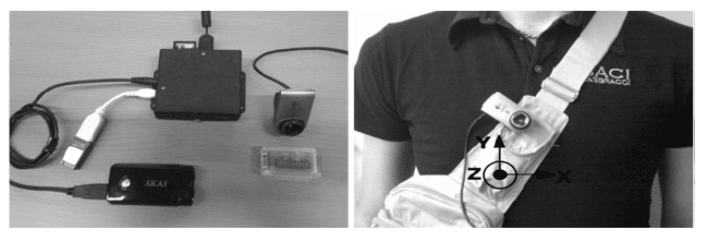
Photographs of the custom chest-mounted systems worn by each subject.
Taken from “Human Activity Recognition from Accelerometer Data Using a Wearable Device”.

The seven activities were performed and recorded by each subject in a continuous sequence.

The specific activities performed were:

• 1: Working at Computer (workingPC).
• 2: Standing Up, Walking and Going up/down stairs.
• 3: Standing (standing).
• 4: Walking (waking).
• 5: Going Up/Down Stairs (stairs).
• 6: Walking and Talking with Someone.
• 7: Talking while Standing (talking).

The paper used a subset of the data, specifically 14 subjects and 5 activities. It is not immediately clear why the other 2 activities (2 and 6) were not used.

Data have been collected from fourteen testers, three women and eleven men with age between 27 and 35. […] The data set collected is composed by 33 minutes of walking up/down stairs, 82 minutes of walking, 115 minutes of talking, 44 minutes of staying standing and 86 minutes of working at computer.

— Human Activity Recognition from Accelerometer Data Using a Wearable Device, 2011.

The focus of the paper was the development of hand-crafted features from the data, and the developing of machine learning algorithms.

Data was split into windows of one second of observations (52) with a 50% overlap between windows.

We extract features from data using windows of 52 samples, corresponding to 1 second of accelerometer data, with 50% of overlapping between windows. From each window, we propose to extract the following features: root mean squared value of integration of acceleration in a window, and mean value of Minmax sums. […] Still, in order to complete the set of features we add features that have proved to be useful for human activity recognition like: mean value, standard deviation, skewness, kurtosis, correlation between each pairwise of accelerometer axis(not including magnitude), energy of coefficients of seven level wavelet decomposition. In this way, we obtain a 319-dimensional feature vector.

— Human Activity Recognition from Accelerometer Data Using a Wearable Device, 2011.

A suite of machine learning models were fit and evaluated using 5-fold cross-validation and achieved an accuracy of 94%.

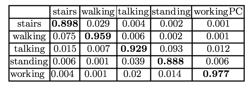
Confusion Matrix of Random Forest evaluated on the dataset.
Taken from “Human Activity Recognition from Accelerometer Data Using a Wearable Device”.

Load Dataset

The dataset can be downloaded directly from the UCI Machine Learning Repository.

• Download Dataset

Unzip the dataset into a new directory called ‘HAR‘.

The directory contains a list of CSV files, one per subject (1-15) and a readme file.

Each file contains 5 columns, the row number, x, y, and z accelerometer readings and a class number from 0 to 7, where class 0 means “no activity” and classes 1-7 correspond to the activities listed in the previous section.

For example, below are the first 5 rows from the file “1.csv“:

To get started, we can load each file as a single NumPy array and drop the first column.

The function below named load_dataset() will load all CSV files in the HAR directory, drop the first column and return a list of 15 NumPy arrays.

The complete example is listed below.

Running the example loads all of the data and prints the number of loaded subjects.

Note, the files in the directory are navigated in file-order, which may not be the same as the subject order, e.g. 10.csv comes before 2.csv in file order. I believe this does not matter in this tutorial.

Now that we know how to load the data, we can explore it with some visualizations.

Plot Traces for a Single Subject

A good first visualization is to plot the data for a single subject.

We can create a figure with a plot for each variable for a given subject, including the x, y, and z accelerometer data, and the associated class class values.

The function plot_subject() below will plot the data for a given subject.

We can tie this together with the data loading in the previous section and plot the data for the first loaded subject.

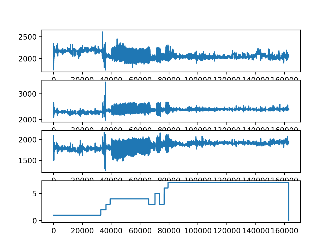
Running the example creates a line plot for each variable for the first loaded subject.

We can see some very large movement in the beginning of the sequence that may be an outlier or unusual behavior that could be removed.

We can also see that the subject performed some actions multiple times. For example, a closer look at the plot of the class variable (bottom plot) suggests the subject performed activities in the following order, 1, 2, 0, 3, 0, 4, 3, 5, 3, 6, 7. Note that activity 3 was performed twice.

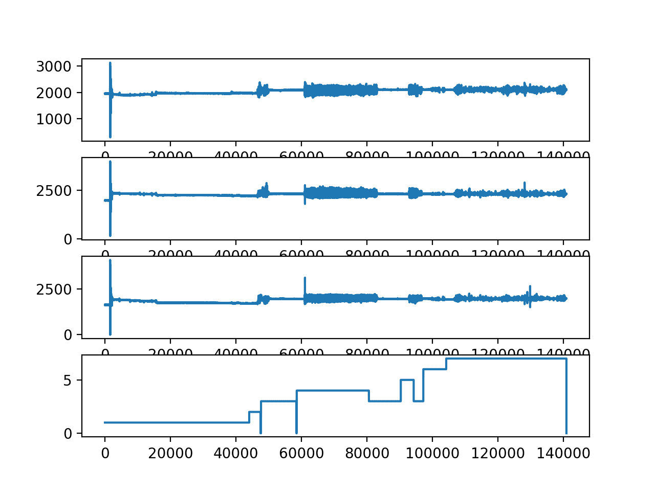
Line plots of x, y, z and class for the first loaded subject.

We can re-run this code and plot the second loaded subject (which might be 10.csv).

Running the example creates a similar plot.

We can see more detail, suggesting that the large outlier seen at the beginning of the previous plot might be washing out values from that subject’s trace.

We see as similar sequence of activities, with activity 3 occurring twice again.

We can also see that some activities are performed for much longer than others. This may impact the ability of a model to discriminate between the activities, e.g. activity 3 (standing) for both subjects has very little data relative to the other activities performed.

Line plots of x, y, z and class for the second loaded subject.

Plot Total Activity Durations

The previous section raised a question around how long or how many observations we have for each activity across all of the subjects.

This may be important if there is a lot more data for one activity than another, suggesting that less-well-represented activities may be harder to model.

We can investigate this by grouping all observations by activity and subject, and plot the distributions. This will give an idea of how long each subject spends performing each activity over the course of their trace.

First, we can group the activities for each subject.

We can do this by creating a dictionary for each subject and store all trace data by activity. The group_by_activity() function below will perform this grouping for each subject.

Next, we can calculate the total duration of each activity for each subject.

We know that the accelerometer data was recorded at 52Hz, so we can divide the lengths of each trace per activity by 52 in order to summarize the durations in seconds.

The function below named plot_durations() will calculate the durations for each activity per subject and plot the results as a boxplot. The box-and-whisker plot is a useful way to summarize the 15 durations per activity as it describes the spread of the durations without assuming a distribution.

The complete example of plotting the distribution of activity durations is listed below.

Running the example plots the distribution of activity durations per subject.

We can see that there is relatively fewer observations for activities 0 (no activity), 2 (standing up, walking and going up/down stairs), 5 (going up/down stairs) and 6 (walking and talking).

This might suggest why activities 2 and 6 were excluded from the experiments in the original paper.

We can also see that each subject spent a lot of time on activity 1 (standing Up, walking and going up/down stairs) and activity 7 (talking while standing). These activities may be over-represented. There may be benefit in preparing model data that undersamples these activities or over samples the other activities.

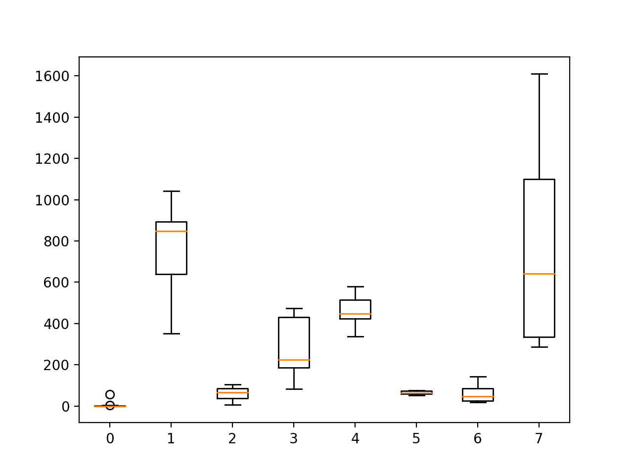
Boxplot of the distribution of activity durations per subject

Plot Traces for Each Subject

Next, it may be interesting to look at the trace data for each subject.

One approach would be to plot all traces for a single subject on a single graph, then line up all graphs vertically. This will allow for a comparison across subjects and across traces within a subject.

The function below named plot_subjects() will plot the accelerometer data for each of the 15 subjects on a separate plot. The trace for each of the x, y, and z data are plotted as orange, green and blue respectively.

The complete example is listed below.

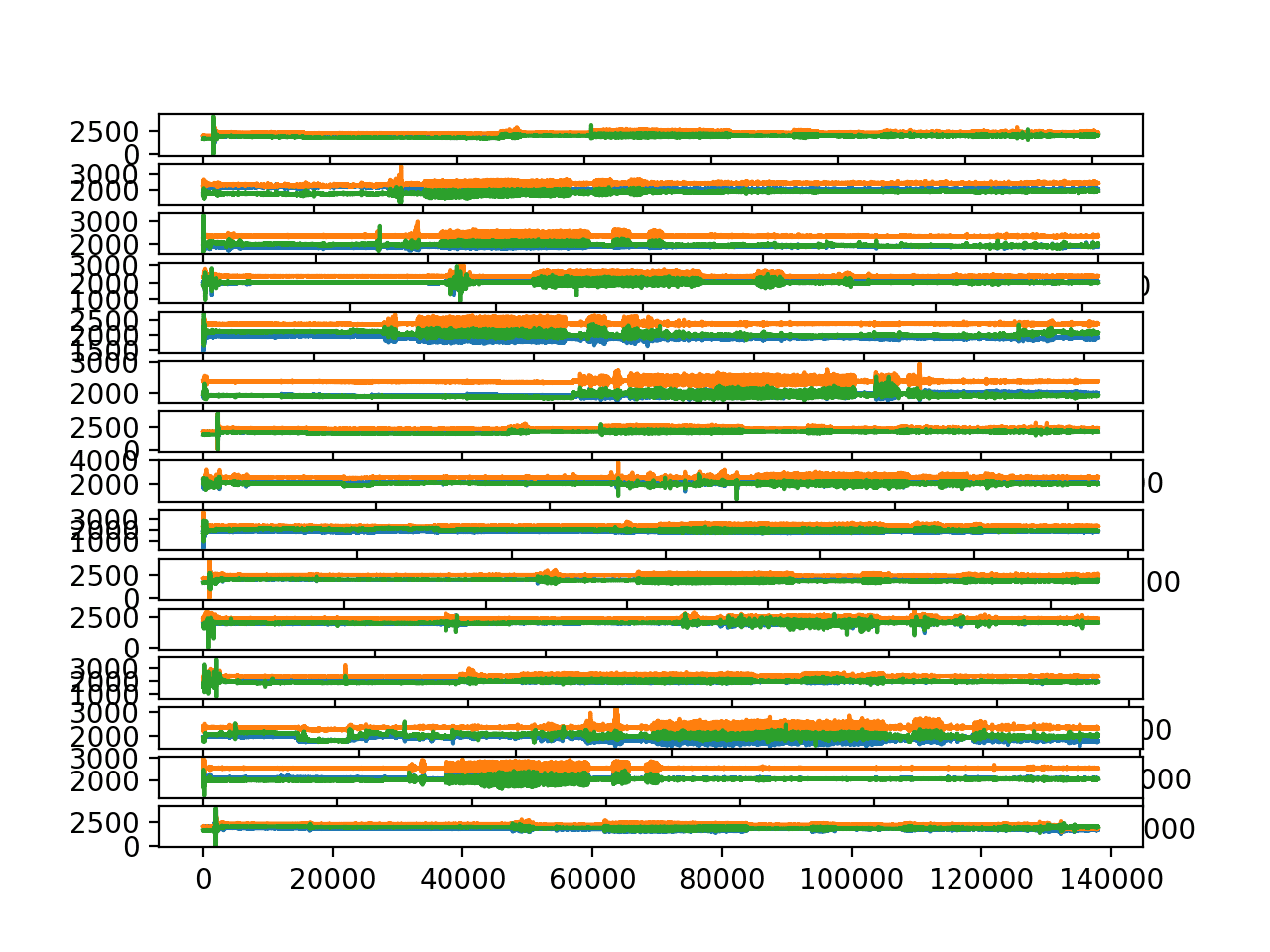
Running the example creates a figure with 15 plots.

We are looking at the general rather than specific trends across the traces.

• We can see lots of orange and green and very little blue, suggesting that perhaps the z data is less important in modeling this problem.
• We can see that the same general change in the trace data at the same times for x and y traces, suggesting that perhaps only a single axis of data may be required to fit a predictive model.
• We can see that each subject has the same large spikes in the trace in the beginning of the sequence (first 60 seconds), perhaps related to the start-up of the experiment.
• We can see similar structures across subjects in the trace data, although some traces appear more muted than others, e.g. compare the amplitude on the first and second plots.

Each subject may have a different full trace length, so direct comparisons by the x-axis may not be reasonable (e.g. performing similar activities at the same time). We are not really concerned with this aspect of the problem anyway.

Line plots of accelerometer trace data for all 15 subjects.

The traces seem to have the same general scale, but the amplitude differences between the subjects suggest that per-subject rescaling of the data might make more sense than cross-subject scaling.

This might make sense for training data, but may be methodologically challenging for scaling the data for a test subject. It would require or assume that the entire trace would be available prior to predicting activities. This would be fine for offline use of a model, but not-online use of the model. It also suggests, that online use of a model might be a lot easier with pre-calibrated trace data (e.g. data coming in at a fixed scale).

Plot Histograms of Trace Observations

The point in the previous section about the possibility of markedly different scales across the different subjects might introduce challenges in modeling this dataset.

We can explore this by plotting a histogram of the distribution of observations for each axis of accelerometer data.

As with the previous section, we can create a plot for each subject, then align the plots for all subjects vertically with the same x-axis to help spot obvious differences in the spreads.

The updated plot_subjects() function for plotting histograms instead of line plots is listed below. The hist() function is used to create a histogram for each axis of accelerometer data, and a large number of bins (100) is used to help spread out the data in the plot. The subplots also all share the same x-axis to aid in the comparison.

The complete example is listed below

Running the example creates a single figure with 15 plots, one for each subject, and 3 histograms on each plot for each of the 3 axis of accelerometer data.

The three colors blue, orange and green represent the x, y and z axises.

This plot suggest that the distribution of each axis of accelerometer is Gaussian or really close to Gaussian. This may help with simple outlier detection and removal along each axis of the accelerometer data.

The plot really helps to show both the relationship between the distributions within a subject and differences in the distributions between the subjects.

Within each subject, a common pattern is for the x (blue) and z (green) are grouped together to the left and y data (orange) is separate to the right. The distribution of y is often sharper where as the distributions of x and z are flatter.

Across subjects, we can see a general clustering of values around 2,000 (whatever the units are), although with a lot of spread. This marked difference in distributions does suggest the need to at least standardize (shift to zero mean and unit variance) the data per axis and per subject before any cross-subject modeling is performed.

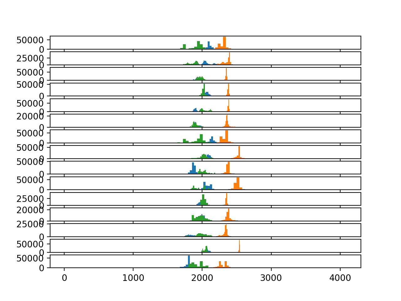
Histograms of accelerometer data for each subject

Approaches to Modeling the Problem

In this section we will explore some ideas and approaches for data preparation and modeling for this problem based on the above exploration of the dataset.

These may help in both modeling this dataset in particular, but also human activity recognition and even time series classification problems in general.

Problem Framing

There are many ways to frame the data as a predictive modeling problem, although all center around the idea of time series classification.

Two main approaches to consider are:

• Per Subject: Model activity classification from trace data per subject.
• Cross Subject: Model activity classification from trace data across subject.

The latter, cross-subject, is more desirable, but the former may also be interesting if the goal is to deeply understand a given subject, e.g. a personalized model within a home.

Two main approaches for framing the data during modeling include:

• Segmented Activities: The trace data can be pre-segmented per activity and a model trained on the entire trace, or features thereof, for each activity.
• Sliding Windows: The contiguous trace for each subject is split into sliding windows, with or without overlap and the mode of each activity for a window is taken as the activity to be predicted.

The former approach may be less realistic in terms of the actual use of the model, but may be an easier problem to model. The latter was the framing of the problem used in the original paper, where 1-second windows were prepared with a 50% overlap.

I fail to see the benefit of the overlap in the framing of the problem, other than doubling the size of the training dataset, that may benefit deep neural networks. In fact, I expect it may result in an overfit model.

Data Preparation

The data suggest some preparation schemes that may be helpful during modeling:

• Down-sampling the accelerometer observations to fractions of a second might be helpful, e.g. 1/4, 1/2, 1, 2 seconds.
• Truncating the first 60 seconds of the raw data might be prudent as it appears to be related to the start-up of the experiment and all subjects are performing activity 1 (working at computer) at that time.
• Using simple outlier detection and removal methods such as values that are 3-to-4 times the standard deviation from the mean for each axis may be useful.
• Perhaps removing activities with relatively fewer observations would be wise, or result in a fairer evaluation of predictive methods (e.g. activities 0, 2, and 6).
• Perhaps rebalancing the activities by oversampling under-represented activities or under-sampling over-represented activities in a training dataset may help with modeling.
• Experimenting with different window sizes would be interesting (e.g. 1, 5, 10, 30 seconds), especially in corroboration with down-sampling of the observations.
• Standardizing the data per subject will almost certainly be required for any cross-subject model. Normalizing data across subjects after per-subject standardization may also be useful.

As noted in a previous section, the standardization of data per-subject does introduce methodological issues, and may be used regardless, defended as the need for calibrated observations from the original hardware system.

Problem Modeling

I would recommend exploring this problem using neural networks.

Unlike the approach used in the paper that used feature engineering and domain-specific hand-crafted features, it would be useful and general to model the raw data directly (downsampled or otherwise).

First, I’d recommend discovering a baseline in performance using a robust method such as random forest or gradient boosting machines. Then explore neural network approaches specifically suited to time series classification problems.

Two types of neural network architectures that might be appropriate are:

• Convolutional Neural Networks or CNNs.
• Recurrent Neural Networks or RNNs, specifically Long Short-Term Memory or LSTMs.

A third is a hybrid of the two:

• CNN LSTMs.

CNNs are able to extract features from input sequences, such as windows of input accelerometer data. RNNs, such as LSTMs are able to learn from long sequences of input data directly, and learn long-term relationships in the data.

I would expect there is little causal relationship in the sequence data, other than each subject looks like they are performing the same artificial sequence of actions, which we would not want to learn. Naively, this might suggest that CNNs would be a better fit for predicting the activity given a sequence of observed accelerometer data.

One-dimensional CNNs have been widely used for this type of problem, with one channel for each axis of the accelerometer data. A good simple starting point would be to fit a CNN model on windows of sequence data directly. This is the approach described in the 2014 paper titled “Convolutional Neural Networks for Human Activity Recognition using Mobile Sensors“, and made clearer with the figure below taken from the paper.

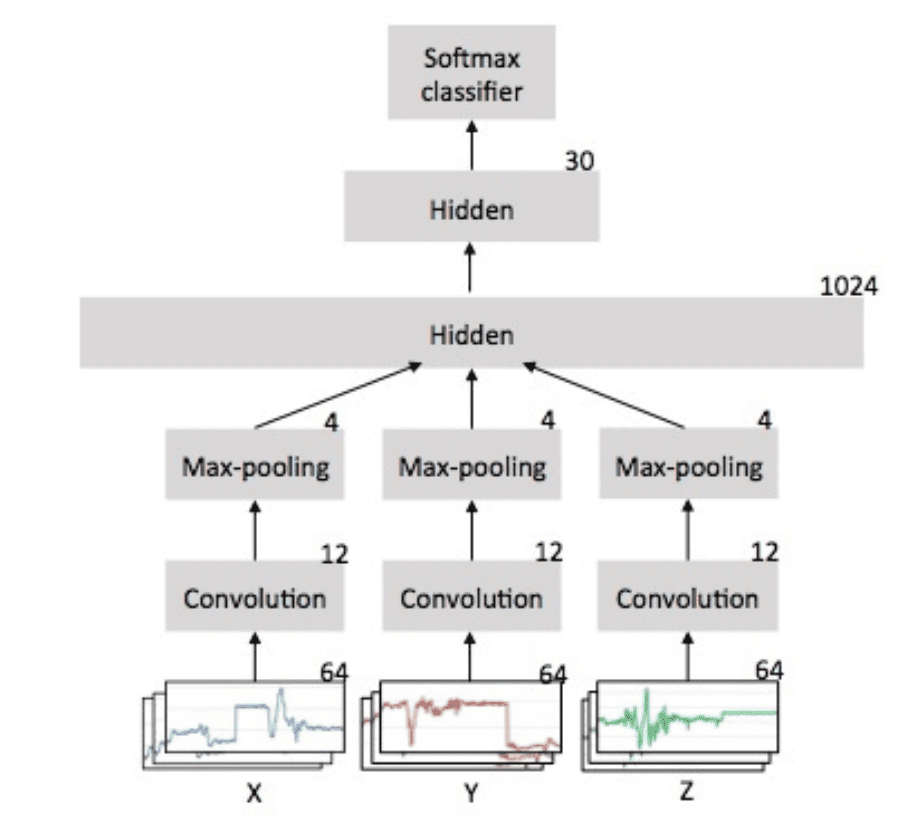
Example of 1D CNN Architecture for Human Activity Recognition
Taken from “Convolutional Neural Networks for Human Activity Recognition using Mobile Sensors”.

A CNN LSTM could be used where the CNN learns a representation for a sub-sequence of observations, then the LSTM learns across these subsequences.

For example, a CNN could distill one second of accelerometer data, this could then be repeated for 30 seconds, to provide 30 time steps of CNN-interpreted data to the LSTM.

I’d expect all three approaches may be interesting on this problem and problems like it.

Model Evaluation

I don’t expect overlapping of the windows would be useful, and in fact might result in minor misleading results if portions of the trace data is available in both train and test dataset during cross-validation. Nevertheless, it would increase the amount of training data.

I think it is important that the data are exposed to the model while maintaining the temporal ordering of the observations. It is possible that multiple windows from a single activity will look similar for a given subject and a random shuffling and separation of windows to train an test data may lead to misleading results.

I would not recommend randomly shuffled k-fold cross-validation was was used in the original paper. I expect that this would lead to optimistic results, with one-second windows of data from all across each the traces of the 15 subjects mixed together for training and testing.

Perhaps a fair evaluation of models in this data would be to use leave-one-out cross validation or LOOCV by subject. This is where a model is fit on the first 14 subjects and evaluated on all windows of the 15th subject. This process is repeated where each subject is given a chance to be used as the hold-out test dataset.

The segmentation of the dataset by subject avoids any issues related to the temporal ordering of individual windows during model evaluation as all windows will are guaranteed new/unseen data.

If you explore any of these modeling ideas, I’d love to know.

Further Reading

This section provides more resources on the topic if you are looking to go deeper.

Papers

• A Comprehensive Study of Activity Recognition Using Accelerometers, 2018
• Deep Learning for Sensor-based Activity Recognition: A Survey, 2017.
• Human Activity Recognition from Accelerometer Data Using a Wearable Device, 2011.
• Convolutional Neural Networks for human activity recognition using mobile sensors, 2014.

API

• sklearn.preprocessing.StandardScaler API
• sklearn.preprocessing.MinMaxScaler API
• keras.utils.to_categorical API
• Keras Convolutional Layers

Articles

• Activity recognition, Wikipedia
• Activity Recognition from Single Chest-Mounted Accelerometer Data Set, UCI Machine Learning Repository.

Summary

In this tutorial, you discovered a standard human activity recognition dataset for time series classification.

Specifically, you learned:

• How to load and prepare human activity recognition time series classification data.
• How to explore and visualize time series classification data in order to generate ideas for modeling.
• A suite of approaches for framing the problem, preparing the data, modeling and evaluating models for human activity recognition.

Do you have any questions?
Ask your questions in the comments below and I will do my best to answer.

Develop Deep Learning models for Time Series Today!

Develop Your Own Forecasting models in Minutes

...with just a few lines of python code

Discover how in my new Ebook:
Deep Learning for Time Series Forecasting

It provides self-study tutorials on topics like:
CNNs, LSTMs, Multivariate Forecasting, Multi-Step Forecasting and much more...

Finally Bring Deep Learning to your Time Series Forecasting Projects

Skip the Academics. Just Results.

See What's Inside