Neural network models are trained using stochastic gradient descent and model weights are updated using the backpropagation algorithm.
The optimization solved by training a neural network model is very challenging and although these algorithms are widely used because they perform so well in practice, there are no guarantees that they will converge to a good model in a timely manner.
The challenge of training neural networks really comes down to the challenge of configuring the training algorithms.
In this post, you will discover tips and tricks for getting the most out of the backpropagation algorithm when training neural network models.
After reading this post, you will know:
The challenge of training a neural network is really the balance between learning the training dataset and generalizing to new examples beyond the training dataset.
Eight specific tricks that you can use to train better neural network models, faster.
Second order optimization algorithms that can also be used to train neural networks under certain circumstances.
Kick-start your project with my new book Better Deep Learning, including step-by-step tutorials and the Python source code files for all examples.
Let’s get started.
8 Tricks for Configuring Backpropagation to Train Better Neural Networks, Faster Photo by Jamesthe1st, some rights reserved.
Post Overview
This tutorial is divided into five parts; they are:
Efficient BackProp Overview
Learning and Generalization
8 Practical Tricks for Backpropagation
Second Order Optimization Algorithms
Discussion and Conclusion
Efficient BackProp Overview
The 1998 book titled “Neural Networks: Tricks of the Trade” provides a collection of chapters by academics and neural network practitioners that describe best practices for configuring and using neural network models.
The book was updated at the cusp of the deep learning renaissance and a second edition was released in 2012 including 13 new chapters.
The chapter was also summarized in a preface in both editions of the book titled “Speed Learning.”
It is an important chapter and document as it provides a near-exhaustive summary of how to best configure backpropagation under stochastic gradient descent as of 1998, and much of the advice is just as relevant today.
In this post, we will focus on this chapter or paper and attempt to distill the most relevant advice for modern deep learning practitioners.
For reference, the chapter is divided into 10 sections; they are:
1.1: Introduction
1.2: Learning and Generalization
1.3: Standard Backpropagation
1.4: A Few Practical Tricks
1.5: Convergence of Gradient Descent
1.6: Classical Second Order Optimization Methods
1.7: Tricks to Compute the Hessian Information in Multilayer Networks
1.8: Analysis of the Hessian in Multi-layer Networks
1.9: Applying Second Order Methods to Multilayer Networks
1.10: Discussion and Conclusion
We will focus on the tips and tricks for configuring backpropagation and stochastic gradient descent.
Want Better Results with Deep Learning?
Take my free 7-day email crash course now (with sample code).
Click to sign-up and also get a free PDF Ebook version of the course.
Learning and Generalization
The chapter begins with a description of the general problem of the dual challenge of learning and generalization with neural network models.
The authors motivate the article by highlighting that the backpropagation algorithm is the most widely used algorithm to train neural network models because it works and because it is efficient.
Backpropagation is a very popular neural network learning algorithm because it is conceptually simple, computationally efficient, and because it often works. However, getting it to work well, and sometimes to work at all, can seem more of an art than a science.
The authors also remind us that training neural networks with backpropagation is really hard. Although the algorithm is both effective and efficient, it requires the careful configuration of multiple model properties and model hyperparameters, each of which requires deep knowledge of the algorithm and experience to set correctly.
And yet, there are no rules to follow to “best” configure a model and training process.
Designing and training a network using backprop requires making many seemingly arbitrary choices such as the number and types of nodes, layers, learning rates, training and test sets, and so forth. These choices can be critical, yet there is no foolproof recipe for deciding them because they are largely problem and data dependent.
The goal of training a neural network model is most challenging because it requires solving two hard problems at once:
Learning the training dataset in order to best minimize the loss.
Generalizing the model performance in order to make predictions on unseen examples.
There is a trade-off between these concerns, as a model that learns too well will generalize poorly, and a model that generalizes well may be underfit. The goal of training a neural network well is to find a happy balance between these two concerns.
This chapter is focused on strategies for improving the process of minimizing the cost function. However, these strategies must be used in conjunction with methods for maximizing the network’s ability to generalize, that is, to predict the correct targets for patterns the learning system has not previously seen.
Interestingly, the problem of training a neural network model is cast in terms of the bias-variance trade-off, often used to describe machine learning algorithms in general.
When fitting a neural network model, these terms can be defined as:
Bias: A measure of how the network output averaged across all datasets differs from the desired function.
Variance: A measure of how much the network output varies across datasets.
This framing casts defining the capacity of the model as a choice of bias, controlling the range of functions that can be learned. It casts variance as a function of the training process and the balance struck between overfitting the training dataset and generalization error.
This framing can also help in understanding the dynamics of model performance during training. That is, from a model with large bias and small variance in the beginning of training to a model with lower bias and higher variance at the end of training.
Early in training, the bias is large because the network output is far from the desired function. The variance is very small because the data has had little influence yet. Late in training, the bias is small because the network has learned the underlying function.
These are the normal dynamics of the model, although when training, we must guard against training the model too much and overfitting the training dataset. This makes the model fragile, pushing the bias down, specializing the model to training examples and, in turn, causing much larger variance.
However, if trained too long, the network will also have learned the noise specific to that dataset. This is referred to as overtraining. In such a case, the variance will be large because the noise varies between datasets.
A focus on the backpropagation algorithm means a focus on “learning” at the expense of temporally ignoring “generalization” that can be addressed later with the introduction of regularization techniques.
A focus on learning means a focus on minimizing loss both quickly (fast learning) and effectively (learning well).
The idea of this chapter, therefore, is to present minimization strategies (given a cost function) and the tricks associated with increasing the speed and quality of the minimization.
8 Practical Tricks for Backpropagation
The focus of the chapter is a sequence of practical tricks for backpropagation to better train neural network models.
There are eight tricks; they are:
1.4.1: Stochastic Versus Batch Learning
1.4.2: Shuffling the Examples
1.4.3: Normalizing the Inputs
1.4.4: The Sigmoid
1.4.5: Choosing Target Values
1.4.6: Initializing the Weights
1.4.7: Choosing Learning Rates
1.4.8: Radial Basis Function vs Sigmoid
The section starts off with a comment that the optimization problem that we are trying to solve with stochastic gradient descent and backpropagation is challenging.
Backpropagation can be very slow particularly for multilayered networks where the cost surface is typically non-quadratic, non-convex, and high dimensional with many local minima and/or flat regions.
The authors go on to highlight that in choosing stochastic gradient descent and the backpropagation algorithms to optimize and update weights, we have no grantees of performance.
There is no formula to guarantee that (1) the network will converge to a good solution, (2) convergence is swift, or (3) convergence even occurs at all.
These comments provide the context for the tricks that also make no guarantees but instead increase the likelihood of finding a better model, faster.
Let’s take a closer look at each trick in turn.
Many of the tricks are focused on sigmoid (s-shaped) activation functions, which are no longer best practice for use in hidden layers, having been replaced by the rectified linear activation function. As such, we will spend less time on sigmoid-related tricks.
Tip #1: Stochastic Versus Batch Learning
This tip highlights the choice between using either stochastic or batch gradient descent when training your model.
Stochastic gradient descent, also called online gradient descent, refers to a version of the algorithm where the error gradient is estimated from a single randomly selected example from the training dataset and the model parameters (weights) are then updated.
It has the effect of training the model fast, although it can result in large, noisy updates to model weights.
Stochastic learning is generally the preferred method for basic backpropagation for the following three reasons:
1. Stochastic learning is usually much faster than batch learning.
2. Stochastic learning also often results in better solutions.
3. Stochastic learning can be used for tracking changes.
Batch gradient descent involves estimating the error gradient using the average from all examples in the training dataset. It is faster to execute and is better understood from a theoretical perspective, but results in slower learning.
Despite the advantages of stochastic learning, there are still reasons why one might consider using batch learning:
1. Conditions of convergence are well understood.
2. Many acceleration techniques (e.g. conjugate gradient) only operate in batch learning.
3. Theoretical analysis of the weight dynamics and convergence rates are simpler.
Generally, the authors recommend using stochastic gradient descent where possible because it offers faster training of the model.
Despite the advantages of batch updates, stochastic learning is still often the preferred method particularly when dealing with very large data sets because it is simply much faster.
They suggest making use of a learning rate decay schedule in order to counter the noisy effect of the weight updates seen during stochastic gradient descent.
… noise, which is so critical for finding better local minima also prevents full convergence to the minimum. […] So in order to reduce the fluctuations we can either decrease (anneal) the learning rate or have an adaptive batch size.
They also suggest using mini-batches of samples to reduce the noise of the weight updates. This is where the error gradient is estimated across a small subset of samples from the training dataset instead of one sample in the case of stochastic gradient descent or all samples in the case of batch gradient descent.
This variation later became known as Mini-Batch Gradient Descent and is the default when training neural networks.
Another method to remove noise is to use “mini-batches”, that is, start with a small batch size and increase the size as training proceeds.
Tip #2: Shuffling the Examples
This tip highlights the importance that the order of examples shown to the model during training has on the training process.
Generally, the authors highlight that the learning algorithm performs better when the next example used to update the model is different from the previous example. Ideally, it is the most different or unfamiliar to the model.
Networks learn the fastest from the most unexpected sample. Therefore, it is advisable to choose a sample at each iteration that is the most unfamiliar to the system.
One simple way to implement this trick is to ensure that successive examples used to update the model parameters are from different classes.
… a very simple trick that crudely implements this idea is to simply choose successive examples that are from different classes since training examples belonging to the same class will most likely contain similar information.
This trick can also be implemented by showing and re-showing examples to the model it gets the most wrong or makes the most error on when making a prediction. This approach can be effective, but can also lead to disaster if the examples that are over-represented during training are outliers.
Choose Examples with Maximum Information Content
1. Shuffle the training set so that successive training examples never (rarely) belong to the same class.
2. Present input examples that produce a large error more frequently than examples that produce a small error
Tip #3: Normalizing the Inputs
This tip highlights the importance of data preparation prior to training a neural network model.
The authors point out that neural networks often learn faster when the examples in the training dataset sum to zero. This can be achieved by subtracting the mean value from each input variable, called centering.
Convergence is usually faster if the average of each input variable over the training set is close to zero.
They also comment that this centering of inputs also improves the convergence of the model when applied to the inputs to hidden layers from prior layers. This is fascinating as it lays the foundation for the Batch Normalization technique developed and made widely popular nearly 15 years later.
Therefore, it is good to shift the inputs so that the average over the training set is close to zero. This heuristic should be applied at all layers which means that we want the average of the outputs of a node to be close to zero because these outputs are the inputs to the next layer
The authors also comment on the need to normalize the spread of the input variables. This can be achieved by dividing the values by their standard deviation. For variables that have a Gaussian distribution, centering and normalizing values in this way means that they will be reduced to a standard Gaussian with a mean of zero and a standard deviation of one.
Scaling speeds learning because it helps to balance out the rate at which the weights connected to the input nodes learn.
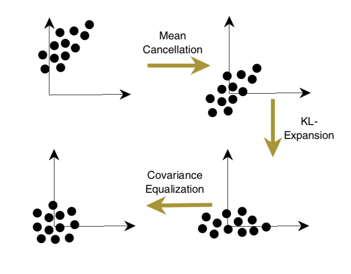
Finally, they suggest de-correlating the input variables. This means removing any linear dependence between the input variables and can be achieved using a Principal Component Analysis as a data transform.
Principal component analysis (also known as the Karhunen-Loeve expansion) can be used to remove linear correlations in inputs
This tip on data preparation can be summarized as follows:
Transforming the Inputs
1. The average of each input variable over the training set should be close to zero.
2. Scale input variables so that their covariances are about the same.
3. Input variables should be uncorrelated if possible.
These recommended three steps of data preparation of centering, normalizing, and de-correlating are summarized nicely in a figure, reproduced from the book below:
Transformation of Inputs Taken from Page 18, “Neural Networks: Tricks of the Trade.”
The centering of input variables may or may not be the best approach when using the more modern ReLU activation functions in the hidden layers of your network, so I’d recommend evaluating both standardization and normalization procedures when preparing data for your model.
Tip #4: The Sigmoid
This tip recommends the use of sigmoid activation functions in the hidden layers of your network.
Nonlinear activation functions are what give neural networks their nonlinear capabilities. One of the most common forms of activation function is the sigmoid …
Specifically, the authors refer to a sigmoid activation function as any S-shaped function, such as the logistic (referred to as sigmoid) or hyperbolic tangent function (referred to as tanh).
Symmetric sigmoids such as hyperbolic tangent often converge faster than the standard logistic function.
The authors recommend modifying the default functions (if needed) so that the midpoint of the function is at zero.
The use of logistic and tanh activation functions for the hidden layers is no longer a sensible default as the performance models that use ReLU converge much faster.
Tip #5: Choosing Target Values
This tip highlights a more careful consideration of the choice of target variables.
In the case of binary classification problems, target variables may be in the set {0, 1} for the limits of the logistic activation function or in the set {-1, 1} for the hyperbolic tangent function when using the cross-entropy or hinge loss functions respectively, even in modern neural networks.
The authors suggest that using values at the extremes of the activation function may make learning the problem more challenging.
Common wisdom might seem to suggest that the target values be set at the value of the sigmoid’s asymptotes. However, this has several drawbacks.
They suggest that achieving values at the point of saturation of the activation function (edges) may require larger and larger weights, which could make the model unstable.
One approach to addressing this is to use target values away from the edge of the output function.
Choose target values at the point of the maximum second derivative on the sigmoid so as to avoid saturating the output units.
I recall that in the 1990s, it was common advice to use target values in the set of {0.1 and 0.9} with the logistic function instead of {0 and 1}.
Tip #6: Initializing the Weights
This tip highlights the importance of the choice of weight initialization scheme and how it is tightly related to the choice of activation function.
In the context of the sigmoid activation function, they suggest that the initial weights for the network should be chosen to activate the function in the linear region (e.g. the line part not the curve part of the S-shape).
The starting values of the weights can have a significant effect on the training process. Weights should be chosen randomly but in such a way that the sigmoid is primarily activated in its linear region.
This advice may also apply to the weight activation for the ReLU where the linear part of the function is positive.
This highlights the important impact that initial weights have on learning, where large weights saturate the activation function, resulting in unstable learning, and small weights result in very small gradients and, in turn, slow learning. Ideally, we seek model weights that are over the linear (non-curvy) part of the activation function.
… weights that range over the sigmoid’s linear region have the advantage that (1) the gradients are large enough that learning can proceed and (2) the network will learn the linear part of the mapping before the more difficult nonlinear part.
The authors suggest a random weight initialization scheme that uses the number of nodes in the previous layer, the so-called fan-in. This is interesting as it is a precursor of what became known as the Xavier weight initialization scheme.
Tip #7: Choosing Learning Rates
This tip highlights the importance of choosing the learning rate.
The learning rate is the amount that the model weights are updated each iteration of the algorithm. A small learning rate can cause slower convergence but perhaps a better result, whereas a larger learning rate can result in faster convergence but perhaps to a less optimal result.
The authors suggest decreasing the learning rate when the weight values begin changing back and forth, e.g. oscillating.
Most of those schemes decrease the learning rate when the weight vector “oscillates”, and increase it when the weight vector follows a relatively steady direction.
They comment that this is a hard strategy when using online gradient descent as, by default, the weights will oscillate a lot.
The authors also recommend using one learning rate for each parameter in the model. The goal is to help each part of the model to converge at the same rate.
… it is clear that picking a different learning rate (eta) for each weight can improve the convergence. […] The main philosophy is to make sure that all the weights in the network converge roughly at the same speed.
They refer to this property as “equalizing the learning speeds” of each model parameter.
Equalize the Learning Speeds
– give each weight its own learning rate
– learning rates should be proportional to the square root of the number of inputs to the unit
– weights in lower layers should typically be larger than in the higher layers
In addition to using a learning rate per parameter, the authors also recommend using momentum and using adaptive learning rates.
It’s interesting that these recommendations later became enshrined in methods like AdaGrad and Adam that are now popular defaults.
Tip #8: Radial Basis Functions vs Sigmoid Units
This final tip is perhaps less relevant today, and I recommend trying radial basis functions (RBF) instead of sigmoid activation functions in some cases.
The authors suggest that training RBF units can be faster than training units using a sigmoid activation.
Unlike sigmoidal units which can cover the entire space, a single RBF unit covers only a small local region of the input space. This can be an advantage because learning can be faster.
Theoretical Grounding
After these tips, the authors go on to provide a theoretical grounding for why many of these tips are a good idea and are expected to result in better or faster convergence when training a neural network model.
Specifically, the tips supported by this analysis are:
Subtract the means from the input variables
Normalize the variances of the input variables.
De-correlate the input variables.
Use a separate learning rate for each weight.
Second Order Optimization Algorithms
The remainer of the chapter focuses on the use of second order optimization algorithms for training neural network models.
This may not be everyone’s cup of tea and requires a background and good memory of matrix calculus. You may want to skip it.
You may recall that the first derivative is the slope of a function (how steep it is) and that backpropagation uses the first derivative to update the models in proportion to their output error. These methods are referred to as first order optimization algorithms, e.g. optimization algorithms that use the first derivative of the error in the output of the model.
You may also recall from calculus that the second order derivative is the rate of change in the first order derivative, or in this case, the gradient of the error gradient itself. It gives an idea of how curved the loss function is for the current set of weights. Algorithms that use the second derivative are referred to as second order optimization algorithms.
The authors go on to introduce five second order optimization algorithms, specifically:
Newton
Conjugate Gradient
Gauss-Newton
Levenberg Marquardt
Quasi-Newton (BFGS)
These algorithms require access to the Hessian matrix or an approximation of the Hessian matrix. You may also recall the Hessian matrix if you covered a theoretical introduction to the backpropagation algorithm. In a hand-wavy way, we use the Hessian to describe the second order derivatives for the model weights.
The authors proceed to outline a number of methods that can be used to approximate the Hessian matrix (for use in second order optimization algorithms), such as: finite difference, square Jacobian approximation, the diagonal of the Hessian, and more.
They then go on to analyze the Hessian in multilayer neural networks and the effectiveness of second order optimization algorithms.
In summary, they highlight that perhaps second order methods are more appropriate for smaller neural network models trained using batch gradient descent.
Classical second-order methods are impractical in almost all useful cases.
Discussion and Conclusion
The chapter ends with a very useful summary of tips for getting the most out of backpropagation when training neural network models.
This summary is reproduced below:
– shuffle the examples
– center the input variables by subtracting the mean
– normalize the input variable to a standard deviation of 1
– if possible, de-correlate the input variables.
– pick a network with the sigmoid function shown in figure 1.4
– set the target values within the range of the sigmoid, typically +1 and -1.
– initialize the weights to random values (as prescribed by 1.16).
Further Reading
This section provides more resources on the topic if you are looking to go deeper.


")


Perfect … love it …
Thanks.
very interesting
Thanks.
Can the second order optimization algorithm configured using python?
Such algorithms are available in Python and are often used in many different scikit-learn algorithms.
“Use a separate learning rate for each weight.”
Whats the method for doing this ?
The adam version of SGD.
tell me about something different training methods of ANN compared with Backpropagation and activation functions.
Hi Ana…The following resource may be of interest to you:
https://medium.com/@sallyrobotics.blog/backpropagation-and-its-alternatives-c09d306aae4c