A Gentle Introduction to Evaluating Limits

The concept of the limit of a function dates back to Greek scholars such as Eudoxus and Archimedes. While they never formally defined limits, many of their calculations were based upon this concept. Isaac Newton formally defined the notion of a limit and Cauchy refined this idea. Limits form the basis of calculus, which in turn defines the foundation of many machine learning algorithms. Hence, it is important to understand how limits of different types of functions are evaluated.

In this tutorial, you will discover how to evaluate the limits of different types of functions.

After completing this tutorial, you will know:

• The different rules for evaluating limits
• How to evaluate the limit of polynomials and rational functions
• How to evaluate the limit of a function with discontinuities
• The Sandwich Theorem

Let’s get started.

A Gentle Introduction to Limits and Continuity Photo by Mehreen Saeed, some rights reserved.

Tutorial Overview

This tutorial is divided into 3 parts; they are:

1. Rules for limits
   1. Examples of evaluating limits using the rules for limits
   2. Limits for polynomials
   3. Limits for rational expressions
2. Limits for functions with a discontinuity
3. The Sandwich Theorem

Rules for Limits

Limits are easy to evaluate if we know a few simple principles, which are listed below. All these rules are based on the known limits of two functions f(x) and g(x), when x approaches a point k:

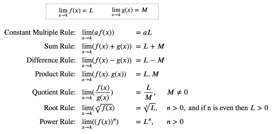
Rules for Evaluating Limits

Examples of Using Rules to Evaluate Limits

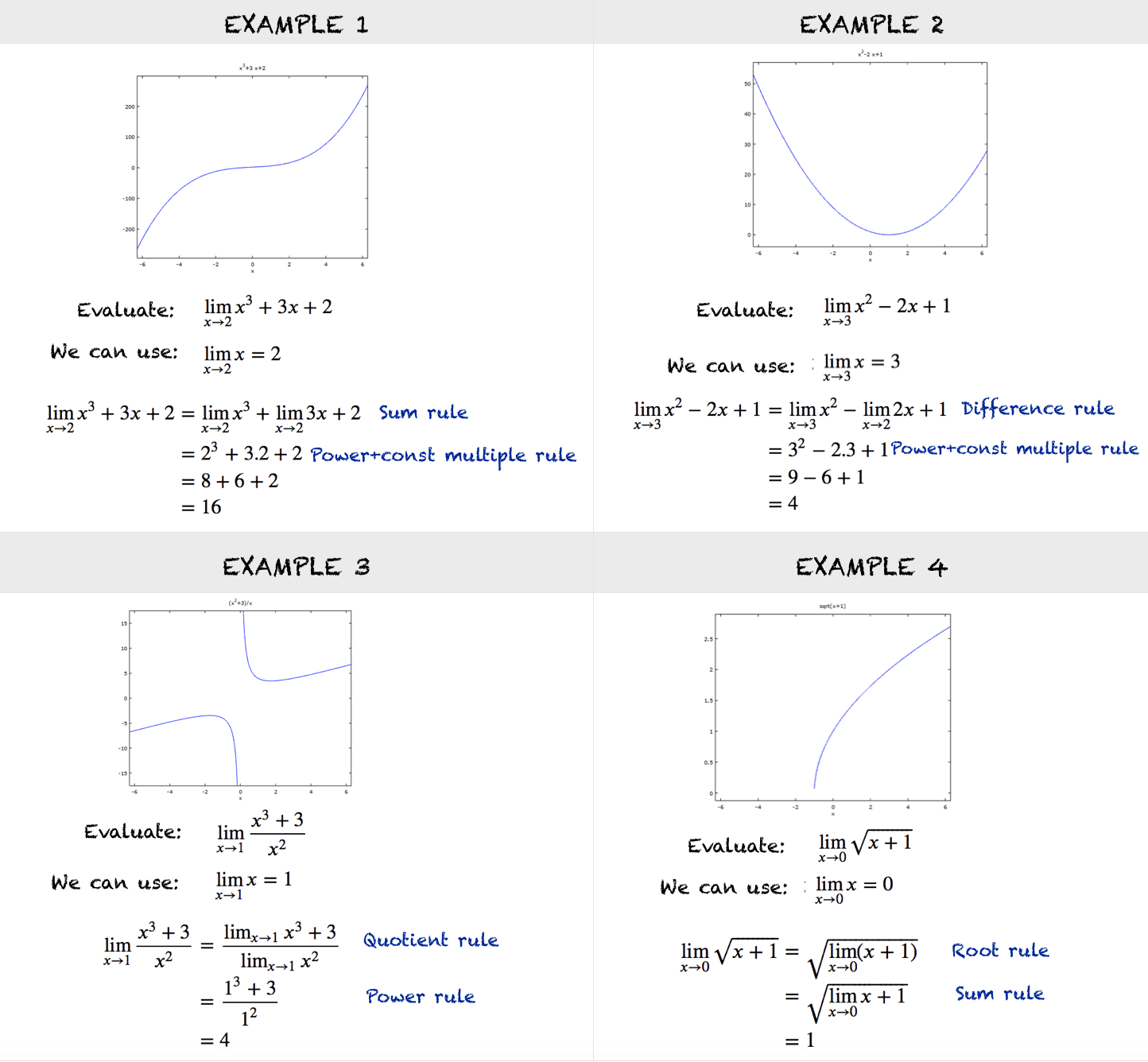
Examples of Evaluating Limits Using Simple Rules

Here are a few examples that use the basic rules to evaluate a limit. Note that these rules apply to functions which are defined at a point as x approaches that point.

Limits for Polynomials

Examples 1 and 2 are that of polynomials. From the rules for limits, we can see that for any polynomial, the limit of the polynomial when x approaches a point k is equal to the value of the polynomial at k. It can be written as: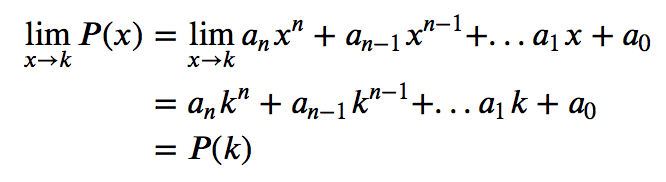

Hence, we can evaluate the limit of a polynomial via direct substitution, e.g.

lim(x→1) x^4+3x^3+2 = 1^4+3(1)^3+2 = 6

Limits for Rational Functions

For rational functions that involve fractions, there are two cases. One case is evaluating the limit when x approaches a point and the function is defined at that point. The other case involves computing the limit when x approaches a point and the function is undefined at that point.

Case 1: Function is Defined

Similar to the case of polynomials, whenever we have a function, which is a rational expression of the form f(x)/g(x) and the denominator is non-zero at a point then:

lim(x→k) f(x)/g(x) = f(k)/g(k) if g(k)≠0

We can therefore evaluate this limit via direct substitution. For example:

lim(x→0)(x^2+1)/(x-1) = -1

Here, we can apply the quotient rule or easier still, substitute x=0 to evaluate the limit. However, this function has no limit when x approaches 1. See the first graph in the figure below.

Case 2: Function is Undefined

Let’s look at another example:

lim(x→2)(x^2-4)/(x-2)

At x=2 we are faced with a problem. The denominator is zero, and hence the function is undefined at x=2. We can see from the figure that the graph of this function and (x+2) is the same, except at the point x=2, where there is a hole. In this case, we can cancel out the common factors and still evaluate the limit for (x→2) as:

lim(x→2)(x^2-4)/(x-2) = lim(x→2)(x-2)(x+2)/(x-2) = lim(x→2)(x+2) = 4

Following image shows the above two examples as well as a third similar example of g_3(x):

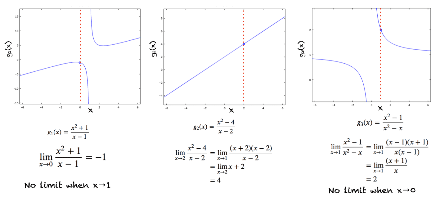
Examples of Computing Limits for Rational Functions

Case for Functions with a Discontinuity

Suppose we have a function h(x), which is defined for all real numbers:

h(x) = (x^2+x)/x,  if x≠0

h(x) = 0, if x=0

The function g(x),  has a discontinuity at x=0, as shown in the figure below. When evaluating lim(x→0)h(x), we have to see what happens to h(x) when x is close to 0 (and not when x=0). As we approach x=0 from either side, h(x) approaches 1, and hence lim(x→0)h(x)=1.

The function m(x) shown in the figure below is another interesting case. This function is also defined for all real numbers but the limit does not exist when x→0.

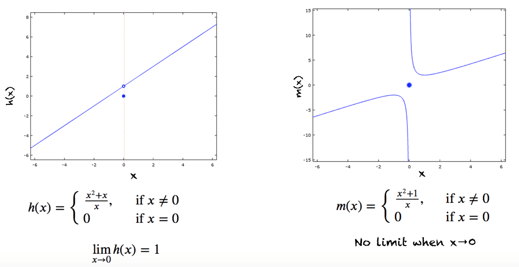
Evaluating Limits when there is a Discontinuity

The Sandwich Theorem

This theorem is also called the Squeeze theorem or the Pinching theorem. It states that when the following are true:

1. x is close to k
2. f(x) <= g(x) <= h(x)
3. lim(x→k)f(x) = lim(x→k)h(x) = L

then the limit of g(x) as x approaches k is given by:

lim(x→k)g(x) = L

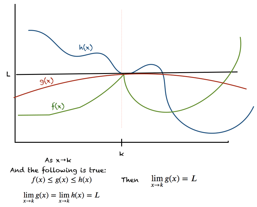
The Sandwich Theorem

This theorem is illustrated in the figure below:

Using this theorem we can evaluate the limits of many complex functions. A well known example involves the sine function:

lim(x→0)x^2sin(1/x)

Computing Limits Using Sandwich Theorem

We know that the sin(x) always alternates between -1 and +1. Using this fact, we can solve this limit as shown below:

Extensions

This section lists some ideas for extending the tutorial that you may wish to explore.

• L’Hospital’s Rule and Indeterminate Forms (requires function derivatives)
• Function derivative defined in terms of the limit of a function
• Function integrals

If you explore any of these extensions, I’d love to know. Post your findings in the comments below.

Further Reading

The best way to learn and understand mathematics is via practice, and solving more problems. This section provides more resources on the topic if you are looking to go deeper.

Tutorials

• Tutorial on limits and continuity
• Additional resources on Calculus Books for Machine Learning

Books

• Thomas’ Calculus, 14th edition, 2017. (based on the original works of George B. Thomas, revised by Joel Hass, Christopher Heil, Maurice Weir)
• Calculus, 3rd Edition, 2017. (Gilbert Strang)
• Calculus, 8th edition, 2015. (James Stewart)

Summary

In this tutorial, you discovered how limits for different types of functions can be evaluated.

Specifically, you learned:

• Rules for evaluating limits for different functions.
• Evaluating limits of polynomials and rational functions
• Evaluating limits when discontinuities are present in a function

Do you have any questions? Ask your questions in the comments below and I will do my best to answer. Enjoy calculus!

Get a Handle on Calculus for Machine Learning!

Feel Smarter with Calculus Concepts

...by getting a better sense on the calculus symbols and terms

Discover how in my new Ebook:
Calculus for Machine Learning

It provides self-study tutorials with full working code on:
differntiation, gradient, Lagrangian mutiplier approach, Jacobian matrix, and much more...

Bring Just Enough Calculus Knowledge to
Your Machine Learning Projects

See What's Inside