
If you have implemented a transformer model in PyTorch, you can use the same code for both training and inference, but in very different ways. During training, you usually process a batch of fixed-length token sequences and update the model weights. During inference, the weights are fixed and the model generates new tokens one at a time.
This difference changes almost everything about performance. Training is dominated by large matrix multiplications and the backward pass. Inference is dominated by repeated forward passes, memory movement, and the need to keep previous attention keys and values available for the next token.
In this chapter, you will learn about:
- The autoregressive generation loop
- The difference between prefill and decode
- Why key-value caching is necessary
- How to implement a simple KV cache
- How to reason about the memory used by the cache
Let’s get started.

Using a Transformer Model: From Training to Inference
Photo by Jacob Smith. Some rights reserved.
Overview
This chapter is divided into four parts; they are:
- Autoregressive Generation
- Prefill and Decode
- A Simple KV Cache
- Memory Usage of the KV Cache
Autoregressive Generation
A decoder-only transformer model predicts the next token from the tokens that came before it. The strict requirement of using only the previous tokens is enforced by the causal attention mechanism. If the input tokens are:
|
1 |
The cat sat on the |
the model returns a probability distribution over the vocabulary for the next token. A likely next token may be “mat”, but the model does not return a word directly. It returns logits, which are unnormalized scores for every token in the vocabulary.
The generation loop is therefore simple:
- Tokenize the prompt.
- Run the model to obtain logits for the next token.
- Choose a token from the logits.
- Append that token to the input.
- Repeat until a stopping rule is reached.
This is called autoregressive generation because each new token depends on the previous generated tokens. The model cannot generate the tenth output token before it knows the first nine output tokens.
A very small greedy decoding loop can be written as follows:
|
1 2 3 4 5 6 7 8 9 10 11 12 13 |
import torch @torch.no_grad() def greedy_decode(model, input_ids, max_new_tokens): output_ids = input_ids.clone() for _ in range(max_new_tokens): logits = model(output_ids) next_token_logits = logits[:, -1, :] next_token = next_token_logits.argmax(dim=-1, keepdim=True) output_ids = torch.cat([output_ids, next_token], dim=1) return output_ids |
In the code above, model is a PyTorch model, max_new_tokens is a positive integer, and all other variables are PyTorch tensors. The for-loop iterates max_new_tokens times, and at each iteration, it feeds the entire sequence back into the model to get the logits for the next token. The argmax() function selects the highest-scoring token. The cat() function is used to concatenate the new token to the output sequence, which will be used in the next iteration until the stopping rule is reached.
This code is easy to understand, but it is inefficient. At every iteration, it feeds the entire sequence back into the model. If the prompt has 1,000 tokens and you generate 100 new tokens, the model repeatedly recomputes the hidden states for the same prompt tokens. The model processes $O(N^2)$ tokens in this function, for a prompt of length $N$.
The actual time complexity of the code is even worse. Without caching, every forward pass recomputes attention for all tokens in the growing sequence. If the sequence length is $N$, self-attention has $O(N^2)$ score computation. For generation, this means you repeat a large amount of work. (Precisely if the output sequence length is $N=P+G$ with prompt length $P$ and number of generated tokens $G$, the computation complexity should be $O(P^2G + PG^2 + G^3)$ naively. With cache, we can reduce it to $O(P^2 + PG)$.)
Inference systems mitigate this by splitting generation into two phases: prefill and decode.
Prefill and Decode
Generation usually begins with a prompt. The prompt is known before generation starts. The model can process all prompt tokens in one forward pass. This is called the prefill phase.
During prefill, the model computes hidden states for all prompt tokens and produces logits for the next token. It also computes keys and values for all attention layers. These keys and values can be saved because they will be needed by every future token.
After the first new token is selected, generation enters the decode phase. In decode, the model receives only the newest token. It computes the query, key, and value for that token, appends the new key and value to the cache, and attends the new query over all cached keys and values.
This changes the cost of one decode step. Instead of recomputing attention for the whole sequence, the model computes attention for only one new query against all previous keys. The per-token attention cost changes from roughly $O(N^2)$ to $O(N)$ for a sequence of length $N$. The prefill step is still $O(N^2)$, but it is performed only once for the prompt.
This distinction is important enough that serving systems usually measure prefill and decode separately:
- Prefill affects time to first token. A slow prefill increases time to the first token.
- Decode affects the speed of streaming output tokens. A slow decode reduces the rate at which output tokens are streamed.
A short prompt with a long answer stresses decode. A long prompt with a short answer stresses prefill. A chat application with a long conversation history stresses both.
The matrix below illustrates the attention-score matrix $QK^\top$. Assume the prompt has five tokens. During prefill, the model computes the $5 \times 5$ block in blue. During decode, one new token is added at a time. Each decode step adds one new row to the matrix, shown in a different shade of red. The elements in black are ignored from calculation due to the causal mask.
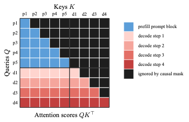
The attention-score matrix grows during generation. Prefill computes the prompt block once (in blue). Each decode iteration appends one row (due to expanded $Q$) and one column (due to expanded $K$) for the newly generated token.
A Simple KV Cache
The KV cache is where the model stores the attention keys and values produced by previous tokens. To see how it works, you do not need a large model. The following code builds a small transformer-like model with a cache.
This model is not intended to produce useful text. Its purpose is to show how the cache is created during prefill and extended during decode.
|
1 2 3 4 5 6 7 8 9 10 11 12 13 14 15 16 17 18 19 20 21 22 23 24 25 26 27 28 29 30 31 32 33 34 35 36 37 38 39 40 41 42 43 44 45 46 47 48 49 50 51 52 53 54 55 56 57 58 59 60 61 62 63 64 65 66 67 68 69 70 71 72 73 74 75 76 77 78 79 80 81 82 83 84 85 86 87 88 89 90 |
import math import torch import torch.nn as nn import torch.nn.functional as F class SelfAttention(nn.Module): def __init__(self, hidden_size, num_heads): super().__init__() assert hidden_size % num_heads == 0 self.num_heads = num_heads self.head_dim = hidden_size // num_heads self.qkv = nn.Linear(hidden_size, 3 * hidden_size) self.out = nn.Linear(hidden_size, hidden_size) def forward(self, x, past_kv=None): # Note: Positional encoding and padding masks are not implemented here batch_size, seq_len, hidden_size = x.shape qkv = self.qkv(x) qkv = qkv.view(batch_size, seq_len, 3, self.num_heads, self.head_dim) qkv = qkv.permute(2, 0, 3, 1, 4) q, k, v = qkv[0], qkv[1], qkv[2] if past_kv is not None: past_k, past_v = past_kv k = torch.cat([past_k, k], dim=2) v = torch.cat([past_v, v], dim=2) total_len = k.size(2) past_len = total_len - seq_len scores = q @ k.transpose(-2, -1) scores = scores / math.sqrt(self.head_dim) # A token may attend to all cached tokens and earlier tokens # in the current chunk, but not future tokens. causal_mask = torch.ones(seq_len, total_len, device=x.device, dtype=torch.bool) causal_mask = torch.tril(causal_mask, diagonal=past_len) scores = scores.masked_fill(~causal_mask, float("-inf")) attn = F.softmax(scores, dim=-1) y = attn @ v y = y.transpose(1, 2).contiguous().view(batch_size, seq_len, hidden_size) return self.out(y), (k, v) class Block(nn.Module): def __init__(self, hidden_size, num_heads): super().__init__() self.attn_norm = nn.LayerNorm(hidden_size) self.attn = SelfAttention(hidden_size, num_heads) self.ffn_norm = nn.LayerNorm(hidden_size) self.ffn = nn.Sequential( nn.Linear(hidden_size, 4 * hidden_size), nn.GELU(), nn.Linear(4 * hidden_size, hidden_size), ) def forward(self, x, past_kv=None): attn_out, new_kv = self.attn(self.attn_norm(x), past_kv=past_kv) x = x + attn_out x = x + self.ffn(self.ffn_norm(x)) return x, new_kv class TinyCausalLM(nn.Module): def __init__(self, vocab_size=128, hidden_size=64, num_heads=4, num_layers=2): super().__init__() self.token_emb = nn.Embedding(vocab_size, hidden_size) self.blocks = nn.ModuleList([ Block(hidden_size, num_heads) for _ in range(num_layers) ]) self.norm = nn.LayerNorm(hidden_size) self.lm_head = nn.Linear(hidden_size, vocab_size, bias=False) def forward(self, input_ids, past_kv=None): x = self.token_emb(input_ids) new_cache = [] if past_kv is None: past_kv = [None] * len(self.blocks) for block, layer_past in zip(self.blocks, past_kv): x, layer_cache = block(x, past_kv=layer_past) new_cache.append(layer_cache) logits = self.lm_head(self.norm(x)) return logits, new_cache |
The cache is a list with one element per transformer layer. Each element is a pair (k, v). The shape of each tensor is:
|
1 |
[batch_size, num_heads, sequence_length, head_dim] |
During prefill, sequence_length is the prompt length. During decode, the model receives one token at a time and appends one position to the cache.
You may notice that only keys and values are stored in the cache but not the query tensor. Note that the forward() method is to produce the next token’s logits. To do so, you only need the last token in the query tensor (which is from the immediate previous token generated) to multiply with every token in the keys to produce attention scores, which are then used to form a weighted sum of the values. That’s why it is only a KV cache while the attention mechanism is a function of query, key, and value.
Here is a minimal generation loop using the cache:
|
1 2 3 4 5 6 7 8 9 10 11 12 13 14 15 16 17 18 19 20 21 22 23 |
torch.no_grad() def greedy_decode_with_cache(model, input_ids, max_new_tokens): output_ids = input_ids.clone() # Prefill: process the whole prompt once. logits, cache = model(input_ids) next_token = logits[:, -1, :].argmax(dim=-1, keepdim=True) output_ids = torch.cat([output_ids, next_token], dim=1) # Decode: process only the most recent token. assert max_new_tokens > 0, "max_new_tokens must be positive" for _ in range(max_new_tokens - 1): logits, cache = model(next_token, past_kv=cache) next_token = logits[:, -1, :].argmax(dim=-1, keepdim=True) output_ids = torch.cat([output_ids, next_token], dim=1) return output_ids model = TinyCausalLM() prompt = torch.tensor([[10, 20, 30, 40]]) generated = greedy_decode_with_cache(model, prompt, max_new_tokens=8) print(generated) |
The model still produces one token at a time. The difference is that it no longer recomputes the prompt tokens after prefill. The key logic is in SelfAttention.forward(): when past_kv is provided, the method appends the new key and value to the cached tensors. During decode, the model processes only the most recently generated next_token rather than the entire sequence. This is the basic idea behind the KV cache in production inference engines.
Memory Usage of the KV Cache
The KV cache saves compute, but it consumes memory. For each token, each layer stores a key tensor and a value tensor. The approximate memory usage is:
|
1 2 |
bytes = 2 * num_layers * batch_size * sequence_length * num_kv_heads * head_dim * bytes_per_element |
The factor of 2 is for keys and values. The num_kv_heads value may be smaller than the number of query heads for models that use multi-query attention or grouped-query attention.
For a model with 32 layers, 32 KV heads, head dimension 128, BF16 cache values, batch size 1, and sequence length 4,096:
|
1 2 3 |
2 * 32 * 1 * 4096 * 32 * 128 * 2 bytes = 2,147,483,648 bytes = 2 GiB |
This is only the KV cache for one request. It does not include model weights, temporary activations, tokenization buffers, or framework overhead. If the service handles many users concurrently, KV cache memory quickly becomes a limiting factor.
For this reason, an inference system must release KV cache memory when a request is finished. A simple script can let Python garbage collection handle this, a production server needs more efficient memory management, typically using cache blocks instead of individual tensors.
The layout of the cache also matters. In the simple code above, each decode step appends tensors using torch.cat(). This is fine for teaching, but it is inefficient because it repeatedly allocates new tensors and copies old data. Real serving engines pre-allocate cache memory in advance or use a paged layout. Later chapters will revisit this issue in detail.
Efficient KV-cache management is a major differentiator among inference systems.
Further Reading
Below are some resources you may find useful:
- Attention Is All You Need, by Vaswani et al.
This is the original Transformer paper. It introduces scaled dot-product attention, multi-head attention, and the query-key-value formulation used throughout this chapter. - Attention (machine learning), on Wikipedia.
This is a useful quick reference for the attention mechanism, including the formula $\operatorname{softmax}(QK^\top / \sqrt{d_k})V$ and the relationship between attention, self-attention, and the Transformer architecture. - Fast Transformer Decoding: One Write-Head is All You Need, by Noam Shazeer.
This paper introduces multi-query attention. It is directly related to inference because it reduces the amount of key and value data that must be read during incremental decoding. - FlashAttention: Fast and Memory-Efficient Exact Attention with IO-Awareness, by Dao et al.
FlashAttention is not only an inference algorithm; the original paper emphasizes faster Transformer training and memory-efficient exact attention. It is still relevant to inference because prompt prefill and long-context attention also benefit from reducing memory traffic and avoiding materializing the full attention matrix. - Orca: A Distributed Serving System for Transformer-Based Generative Models, by Yu et al.
This paper focuses on inference serving. It introduces iteration-level scheduling and selective batching, which are important ideas behind continuous batching for autoregressive generation. - Efficient Memory Management for Large Language Model Serving with PagedAttention, by Kwon et al.
This paper is directly about LLM inference serving. PagedAttention stores the KV cache in fixed-size blocks instead of requiring each request’s cache to be contiguous, reducing memory fragmentation and allowing larger batches.
Summary
In this article, you learned that inference is not just training without the backward pass. The model is used in a different pattern: one prefill step followed by many decode steps. The KV cache avoids recomputing attention keys and values for previous tokens, changing the per-token attention cost during decode from quadratic to linear in the sequence length.
You also implemented a simple KV cache in a tiny transformer model. This cache is the foundation for many later optimizations, including paged attention, continuous batching, prefix caching, long-context inference, and disaggregated prefill and decode.






No comments yet.