A deep learning model in its simplest form are layers of perceptrons connected in tandem. Without any activation functions, they are just matrix multiplications with limited power, regardless how many of them. Activation is the magic why neural network can be an approximation to a wide variety of non-linear function. In PyTorch, there are many activation functions available for use in your deep learning models. In this post, you will see how the choice of activation functions can impact the model. Specifically,
- What are the common activation functions
- What are the nature of activation functions
- How the different activation functions impact the learning rate
- How the selection of activation function can solve the vanishing gradient problem
Kick-start your project with my book Deep Learning with PyTorch. It provides self-study tutorials with working code.
Let’s get started.

Using Activation Functions in Deep Learning Models
Photo by SHUJA OFFICIAL. Some rights reserved.
Overview
This post is in three parts; they are
- A Toy Model of Binary Classification
- Why Nonlinear Functions?
- The Effect of Activation Functions
A Toy Model of Binary Classification
Let’s start with a simple example of binary classification. Here you use the make_circle() function from scikit-learn to create a synthetic dataset for binary classification. This dataset has two features: The x- and y-coordinate of points. Each point belongs to one of the two classes. You can generate 1000 data points and visualize them as below:
|
1 2 3 4 5 6 7 8 9 10 11 12 13 14 |
from sklearn.datasets import make_circles import matplotlib.pyplot as plt import torch import torch.nn as nn import torch.optim as optim # Make data: Two circles on x-y plane as a classification problem X, y = make_circles(n_samples=1000, factor=0.5, noise=0.1) X = torch.tensor(X, dtype=torch.float32) y = torch.tensor(y.reshape(-1, 1), dtype=torch.float32) plt.figure(figsize=(8,6)) plt.scatter(X[:,0], X[:,1], c=y) plt.show() |
The dataset is visualized as follows: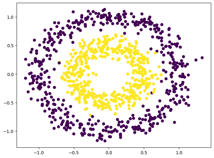
This dataset is special because it is simple but not linearly separable: It is impossible to find a straight line to separate two classes. How can your neural network figure out there’s a circle boundary between the classes is a challenge.
Let’s create a deep learning model for this problem. To make things simple, you do not do cross validation. You may find the neural network overfit the data but it doesn’t affect the discussion below. The model has 4 hidden layers and the output layer gives a sigmodal value (0 to 1) for binary classification. The model accepts a parameter at its constructor to specify what is the activation to use in the hidden layers. You implement the training loop in a function as you will run this for several times.
The implementation is as follows:
|
1 2 3 4 5 6 7 8 9 10 11 12 13 14 15 16 17 18 19 20 21 22 23 24 25 26 27 28 29 30 31 32 33 34 35 36 37 38 39 40 41 42 43 44 45 46 47 48 49 50 51 52 53 |
class Model(nn.Module): def __init__(self, activation=nn.ReLU): super().__init__() self.layer0 = nn.Linear(2,5) self.act0 = activation() self.layer1 = nn.Linear(5,5) self.act1 = activation() self.layer2 = nn.Linear(5,5) self.act2 = activation() self.layer3 = nn.Linear(5,5) self.act3 = activation() self.layer4 = nn.Linear(5,1) self.act4 = nn.Sigmoid() def forward(self, x): x = self.act0(self.layer0(x)) x = self.act1(self.layer1(x)) x = self.act2(self.layer2(x)) x = self.act3(self.layer3(x)) x = self.act4(self.layer4(x)) return x def train_loop(model, X, y, n_epochs=300, batch_size=32): loss_fn = nn.BCELoss() optimizer = optim.Adam(model.parameters(), lr=0.0001) batch_start = torch.arange(0, len(X), batch_size) bce_hist = [] acc_hist = [] for epoch in range(n_epochs): # train model with optimizer model.train() for start in batch_start: X_batch = X[start:start+batch_size] y_batch = y[start:start+batch_size] y_pred = model(X_batch) loss = loss_fn(y_pred, y_batch) optimizer.zero_grad() loss.backward() optimizer.step() # evaluate BCE and accuracy at end of each epoch model.eval() with torch.no_grad(): y_pred = model(X) bce = float(loss_fn(y_pred, y)) acc = float((y_pred.round() == y).float().mean()) bce_hist.append(bce) acc_hist.append(acc) # print metrics every 10 epochs if (epoch+1) % 10 == 0: print("Before epoch %d: BCE=%.4f, Accuracy=%.2f%%" % (epoch+1, bce, acc*100)) return bce_hist, acc_hist |
At the end of each epoch in the training function, you evaluate the model with the entire dataset. The evaluation result is returned when the training finished. In the following, you create a model, train it, and plot the training history. The activation function you use is rectified linear unit or ReLU, which is the most common activation function nowadays:
|
1 2 3 4 5 6 7 8 9 10 |
activation = nn.ReLU model = Model(activation=activation) bce_hist, acc_hist = train_loop(model, X, y) plt.plot(bce_hist, label="BCE") plt.plot(acc_hist, label="Accuracy") plt.xlabel("Epochs") plt.ylim(0, 1) plt.title(str(activation)) plt.legend() plt.show() |
Running this give you the following:
|
1 2 3 4 5 6 7 |
Before epoch 10: BCE=0.7025, Accuracy=50.00% Before epoch 20: BCE=0.6990, Accuracy=50.00% Before epoch 30: BCE=0.6959, Accuracy=50.00% ... Before epoch 280: BCE=0.3051, Accuracy=96.30% Before epoch 290: BCE=0.2785, Accuracy=96.90% Before epoch 300: BCE=0.2543, Accuracy=97.00% |
and this plot: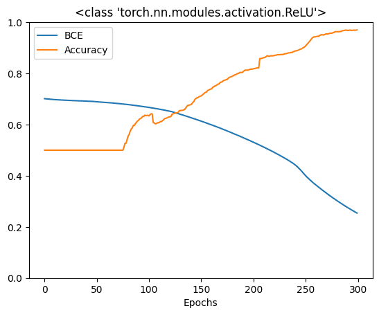
This model works great. After 300 epochs, it can achieve 90% accuracy. However, ReLU is not the only activation function. Historically, sigmoid function and hyperbolic tangents were common in neural networks literatures. If you’re curious, below are how you can compare these three activation functions, using matplotlib:
|
1 2 3 4 5 6 7 8 9 10 11 |
x = torch.linspace(-4, 4, 200) relu = nn.ReLU()(x) tanh = nn.Tanh()(x) sigmoid = nn.Sigmoid()(x) plt.plot(x, sigmoid, label="sigmoid") plt.plot(x, tanh, label="tanh") plt.plot(x, relu, label="ReLU") plt.ylim(-1.5, 2) plt.legend() plt.show() |
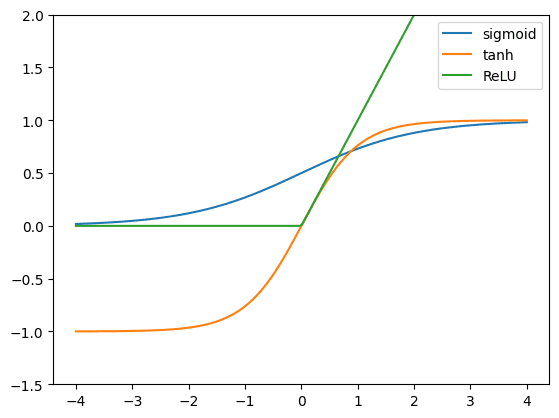
ReLU is called rectified linear unit because it is a linear function $y=x$ at positive $x$ but remains zero if $x$ is negative. Mathematically, it is $y=\max(0, x)$. Hyperbolic tangent ($y=\tanh(x)=\dfrac{e^x – e^{-x}}{e^x+e^{-x}}$) goes from -1 to +1 smoothly while sigmoid function ($y=\sigma(x)=\dfrac{1}{1+e^{-x}}$) goes from 0 to +1.
If you try to differentiate these functions, you will find that ReLU is the easiest: The gradient is 1 at positive region and 0 otherwise. Hyperbolic tangent has a steeper slope therefore its gradient is greater than that of sigmoid function.
All these functions are increasing. Therefore, their gradients are never negative. This is one of the criteria for an activation function suitable to use in neural networks.
Want to Get Started With Deep Learning with PyTorch?
Take my free email crash course now (with sample code).
Click to sign-up and also get a free PDF Ebook version of the course.
Why Nonlinear Functions?
You might be wondering, why all this hype about nonlinear activation functions? Or why can’t we just use an identity function after the weighted linear combination of activations from the previous layer? Using multiple linear layers is basically the same as using a single linear layer. This can be seen through a simple example. Let’s say you have a one hidden layer neural network, each with two hidden neurons.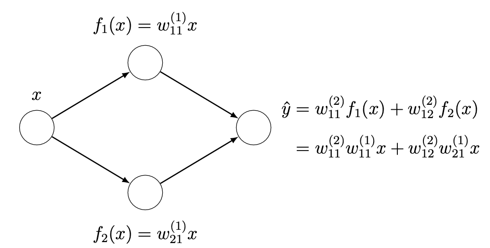
You can then rewrite the output layer as a linear combination of the original input variable if you used a linear hidden layer. If you had more neurons and weights, the equation would be a lot longer with more nesting and more multiplications between successive layer weights. However, the idea remains the same: You can represent the entire network as a single linear layer. To make the network represent more complex functions, you would need nonlinear activation functions.
The Effect of Activation Functions
To explain how much impact the activation function can bring to your model, let’s modify the training loop function to capture more data: The gradients in each training step. You model has four hidden layers and one output layer. In each step, the backward pass calculates the gradient of the weights of each layer and the weight update is done by the optimizer based on the result of the backward pass. You should observe how the gradient changes as the training progressed. Therefore, the training loop function is modified to collect the mean absolute value of the gradient in each layer in each step, as follows:
|
1 2 3 4 5 6 7 8 9 10 11 12 13 14 15 16 17 18 19 20 21 22 23 24 25 26 27 28 29 30 31 32 33 34 35 36 37 38 39 40 |
def train_loop(model, X, y, n_epochs=300, batch_size=32): loss_fn = nn.BCELoss() optimizer = optim.Adam(model.parameters(), lr=0.0001) batch_start = torch.arange(0, len(X), batch_size) bce_hist = [] acc_hist = [] grad_hist = [[],[],[],[],[]] for epoch in range(n_epochs): # train model with optimizer model.train() layer_grad = [[],[],[],[],[]] for start in batch_start: X_batch = X[start:start+batch_size] y_batch = y[start:start+batch_size] y_pred = model(X_batch) loss = loss_fn(y_pred, y_batch) optimizer.zero_grad() loss.backward() optimizer.step() # collect mean absolute value of gradients layers = [model.layer0, model.layer1, model.layer2, model.layer3, model.layer4] for n,layer in enumerate(layers): mean_grad = float(layer.weight.grad.abs().mean()) layer_grad[n].append(mean_grad) # evaluate BCE and accuracy at end of each epoch model.eval() with torch.no_grad(): y_pred = model(X) bce = float(loss_fn(y_pred, y)) acc = float((y_pred.round() == y).float().mean()) bce_hist.append(bce) acc_hist.append(acc) for n, grads in enumerate(layer_grad): grad_hist[n].append(sum(grads)/len(grads)) # print metrics every 10 epochs if epoch % 10 == 9: print("Epoch %d: BCE=%.4f, Accuracy=%.2f%%" % (epoch, bce, acc*100)) return bce_hist, acc_hist, layer_grad |
At the end of the inner for-loop, the gradients of the layer weights are computed by the backward process earlier and you can access to the gradient using model.layer0.weight.grad. Like the weights, the gradients are tensors. You take the absolute value of each element and then compute the mean over all elements. This value depends on the batch and can be very noisy. Thus you summarize all such mean absolute value over the same epoch at the end.
Note that you have five layers in the neural network (hidden and output layers combined). So you can see the pattern of each layer’s gradient across the epochs if you visualize them. In below, you run the training loop as before and plot both the cross entropy and accuracy as well as the mean absolute gradient of each layer:
|
1 2 3 4 5 6 7 8 9 10 11 12 13 14 15 16 |
activation = nn.ReLU model = Model(activation=activation) bce_hist, acc_hist, grad_hist = train_loop(model, X, y) fig, ax = plt.subplots(1, 2, figsize=(12, 5)) ax[0].plot(bce_hist, label="BCE") ax[0].plot(acc_hist, label="Accuracy") ax[0].set_xlabel("Epochs") ax[0].set_ylim(0, 1) for n, grads in enumerate(grad_hist): ax[1].plot(grads, label="layer"+str(n)) ax[1].set_xlabel("Epochs") fig.suptitle(str(activation)) ax[0].legend() ax[1].legend() plt.show() |
Running the above produces the following plot:
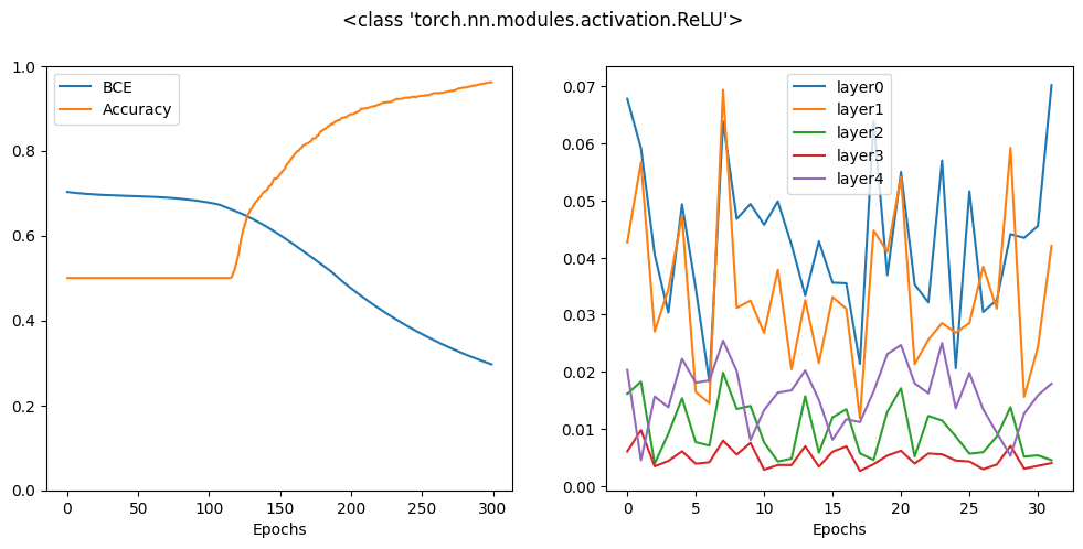
In the plot above, you can see how the accuracy increases and the cross entropy loss decreases. At the same time, you can see the gradient of each layer is fluctuating in a similar range, especially you should pay attention to the line corresponding to the first layer and the last layer. This behavior is ideal.
Let’s repeat the same with a sigmoid activation:
|
1 2 3 4 5 6 7 8 9 10 11 12 13 14 15 16 |
activation = nn.Sigmoid model = Model(activation=activation) bce_hist, acc_hist, grad_hist = train_loop(model, X, y) fig, ax = plt.subplots(1, 2, figsize=(12, 5)) ax[0].plot(bce_hist, label="BCE") ax[0].plot(acc_hist, label="Accuracy") ax[0].set_xlabel("Epochs") ax[0].set_ylim(0, 1) for n, grads in enumerate(grad_hist): ax[1].plot(grads, label="layer"+str(n)) ax[1].set_xlabel("Epochs") fig.suptitle(str(activation)) ax[0].legend() ax[1].legend() plt.show() |
which the plot is as follows: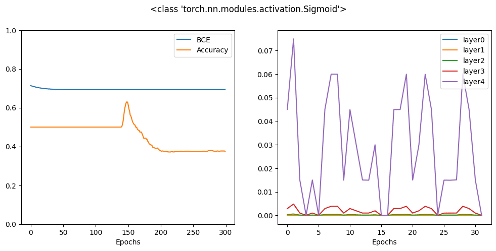
You can see that after 300 epochs, the final result is much worse than ReLU activation. Indeed, you may need much more epochs for this model to converge. The reason can be easily found on the graph at right, which you can see the gradient is significant only for the output layer while all the hidden layers’ gradients are virtually zero. This is the vanishing gradient effect which is the problem of many neural network models with sigmoid activation function.
The hyperbolic tangent function has a similar shape as sigmoid function but its curve is steeper. Let’s see how it behaves:
|
1 2 3 4 5 6 7 8 9 10 11 12 13 14 15 16 |
activation = nn.Tanh model = Model(activation=activation) bce_hist, acc_hist, grad_hist = train_loop(model, X, y) fig, ax = plt.subplots(1, 2, figsize=(12, 5)) ax[0].plot(bce_hist, label="BCE") ax[0].plot(acc_hist, label="Accuracy") ax[0].set_xlabel("Epochs") ax[0].set_ylim(0, 1) for n, grads in enumerate(grad_hist): ax[1].plot(grads, label="layer"+str(n)) ax[1].set_xlabel("Epochs") fig.suptitle(str(activation)) ax[0].legend() ax[1].legend() plt.show() |
Which is: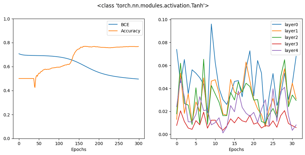
The result looks better than sigmoid activation but still worse then ReLU. In fact, from the gradient plot, you can notice that the gradients at the hidden layers are significant but the gradient at the first hidden layer is obviously at an order of magnitude less than that at the output layer. Thus the backward process is not very effective at propagating the gradient to the input.
This is the reason you see ReLU activation in every neural network model today. Not only because ReLU is simpler and computing the differentiation of it is much faster than the other activation function, but also because it can make the model converge faster.
Indeed, you can do better than ReLU sometimes. In PyTorch, you have a number of ReLU variations. Let’s look at two of them. You can compare these three varation of ReLU as follows:
|
1 2 3 4 5 6 7 8 9 10 |
x = torch.linspace(-8, 8, 200) relu = nn.ReLU()(x) relu6 = nn.ReLU6()(x) leaky = nn.LeakyReLU()(x) plt.plot(x, relu, label="ReLU") plt.plot(x, relu6, label="ReLU6") plt.plot(x, leaky, label="LeakyReLU") plt.legend() plt.show() |
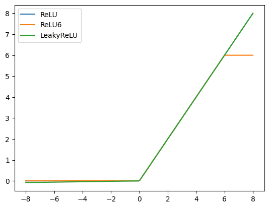 First is the ReLU6, which is ReLU but cap the function at 6.0 if the input to the function is more than 6.0:
|
1 2 3 4 5 6 7 8 9 10 11 12 13 14 15 16 |
activation = nn.ReLU6 model = Model(activation=activation) bce_hist, acc_hist, grad_hist = train_loop(model, X, y) fig, ax = plt.subplots(1, 2, figsize=(12, 5)) ax[0].plot(bce_hist, label="BCE") ax[0].plot(acc_hist, label="Accuracy") ax[0].set_xlabel("Epochs") ax[0].set_ylim(0, 1) for n, grads in enumerate(grad_hist): ax[1].plot(grads, label="layer"+str(n)) ax[1].set_xlabel("Epochs") fig.suptitle(str(activation)) ax[0].legend() ax[1].legend() plt.show() |
 Next is leaky ReLU, which the negative half of ReLU is no longer flat but a gently slanted line. The rationale behind is to keep a small positive gradient at that region.
|
1 2 3 4 5 6 7 8 9 10 11 12 13 14 15 16 |
activation = nn.LeakyReLU model = Model(activation=activation) bce_hist, acc_hist, grad_hist = train_loop(model, X, y) fig, ax = plt.subplots(1, 2, figsize=(12, 5)) ax[0].plot(bce_hist, label="BCE") ax[0].plot(acc_hist, label="Accuracy") ax[0].set_xlabel("Epochs") ax[0].set_ylim(0, 1) for n, grads in enumerate(grad_hist): ax[1].plot(grads, label="layer"+str(n)) ax[1].set_xlabel("Epochs") fig.suptitle(str(activation)) ax[0].legend() ax[1].legend() plt.show() |
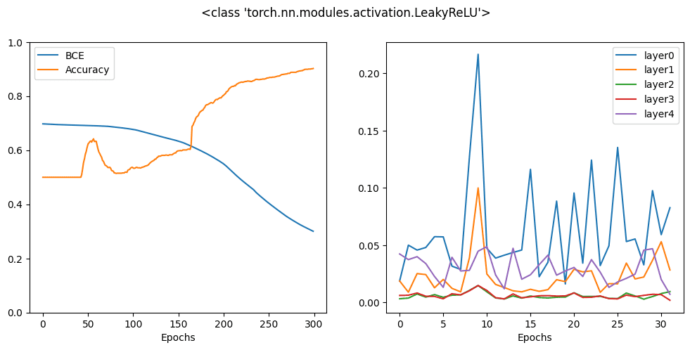
You can see that all these variations can give you similar accuracy after 300 epochs but from the history curve, you know some are faster to reach a high accuracy than another. This is because of the interaction between the gradient of an activation function with the optimizer. There’s no golden rule that a single activation function works best but the design helps:
- in backpropagation, passing the loss metric from the output layer all the way to the input layer
- maintaining stable gradient calculation under specific condition, e.g., limiting floating point precision
- providing enough contrast on different input such that the backward pass can determine accurate adjustment to the parameter
The following is the complete code to generate all the plots above:
|
1 2 3 4 5 6 7 8 9 10 11 12 13 14 15 16 17 18 19 20 21 22 23 24 25 26 27 28 29 30 31 32 33 34 35 36 37 38 39 40 41 42 43 44 45 46 47 48 49 50 51 52 53 54 55 56 57 58 59 60 61 62 63 64 65 66 67 68 69 70 71 72 73 74 75 76 77 78 79 80 81 82 83 84 85 86 87 88 89 90 91 92 93 |
from sklearn.datasets import make_circles import matplotlib.pyplot as plt import torch import torch.nn as nn import torch.optim as optim # Make data: Two circles on x-y plane as a classification problem X, y = make_circles(n_samples=1000, factor=0.5, noise=0.1) X = torch.tensor(X, dtype=torch.float32) y = torch.tensor(y.reshape(-1, 1), dtype=torch.float32) # Binary classification model class Model(nn.Module): def __init__(self, activation=nn.ReLU): super().__init__() self.layer0 = nn.Linear(2,5) self.act0 = activation() self.layer1 = nn.Linear(5,5) self.act1 = activation() self.layer2 = nn.Linear(5,5) self.act2 = activation() self.layer3 = nn.Linear(5,5) self.act3 = activation() self.layer4 = nn.Linear(5,1) self.act4 = nn.Sigmoid() def forward(self, x): x = self.act0(self.layer0(x)) x = self.act1(self.layer1(x)) x = self.act2(self.layer2(x)) x = self.act3(self.layer3(x)) x = self.act4(self.layer4(x)) return x # train the model and produce history def train_loop(model, X, y, n_epochs=300, batch_size=32): loss_fn = nn.BCELoss() optimizer = optim.Adam(model.parameters(), lr=0.0001) batch_start = torch.arange(0, len(X), batch_size) bce_hist = [] acc_hist = [] grad_hist = [[],[],[],[],[]] for epoch in range(n_epochs): # train model with optimizer model.train() layer_grad = [[],[],[],[],[]] for start in batch_start: X_batch = X[start:start+batch_size] y_batch = y[start:start+batch_size] y_pred = model(X_batch) loss = loss_fn(y_pred, y_batch) optimizer.zero_grad() loss.backward() optimizer.step() # collect mean absolute value of gradients layers = [model.layer0, model.layer1, model.layer2, model.layer3, model.layer4] for n,layer in enumerate(layers): mean_grad = float(layer.weight.grad.abs().mean()) layer_grad[n].append(mean_grad) # evaluate BCE and accuracy at end of each epoch model.eval() with torch.no_grad(): y_pred = model(X) bce = float(loss_fn(y_pred, y)) acc = float((y_pred.round() == y).float().mean()) bce_hist.append(bce) acc_hist.append(acc) for n, grads in enumerate(layer_grad): grad_hist[n].append(sum(grads)/len(grads)) # print metrics every 10 epochs if epoch % 10 == 9: print("Epoch %d: BCE=%.4f, Accuracy=%.2f%%" % (epoch, bce, acc*100)) return bce_hist, acc_hist, layer_grad # pick different activation functions and compare the result visually for activation in [nn.Sigmoid, nn.Tanh, nn.ReLU, nn.ReLU6, nn.LeakyReLU]: model = Model(activation=activation) bce_hist, acc_hist, grad_hist = train_loop(model, X, y) fig, ax = plt.subplots(1, 2, figsize=(12, 5)) ax[0].plot(bce_hist, label="BCE") ax[0].plot(acc_hist, label="Accuracy") ax[0].set_xlabel("Epochs") ax[0].set_ylim(0, 1) for n, grads in enumerate(grad_hist): ax[1].plot(grads, label="layer"+str(n)) ax[1].set_xlabel("Epochs") fig.suptitle(str(activation)) ax[0].legend() ax[1].legend() plt.show() |
Further Readings
This section provides more resources on the topic if you are looking to go deeper.
- nn.Sigmoid from PyTorch documentation
- nn.Tanh from PyTorch documentation
- nn.ReLU from PyTorch documentation
- nn.ReLU6 from PyTorch documentation
- nn.LeakyReLU from PyTorch documentation
- Vanishing gradient problem, Wikipedia
Summary
In this chapter, you discovered how to select activation functions for your PyTorch model. You learned:
- What are the common activation functions and how they look like
- How to use activation functions in your PyTorch model
- What is vanishing gradient problem
- The impact of activation function to the performance of your model
Get Started on Deep Learning with PyTorch!

Learn how to build deep learning models
...using the newly released PyTorch 2.0 library
Discover how in my new Ebook:
Deep Learning with PyTorch
It provides self-study tutorials with hundreds of working code to turn you from a novice to expert. It equips you with
tensor operation, training, evaluation, hyperparameter optimization,
and much more...


Hi,
This is very useful tutorial for me thank you very much!
But these 2 statements are not clear for me can you explain further please
1) in backpropagation, passing the loss metric from the output layer all the way to the input layer
2) maintaining stable gradient calculation under specific condition, e.g., limiting floating point precision
Hi Evren…You are very welcome! The following resource may be of interest to you:
https://machinelearningmastery.com/implement-backpropagation-algorithm-scratch-python/