As neural networks become increasingly popular in the field of machine learning, it is important to understand the role that activation functions play in their implementation. In this article, you’ll explore the concept of activation functions that are applied to the output of each neuron in a neural network to introduce non-linearity into the model. Without activation functions, neural networks would simply be a series of linear transformations, which would limit their ability to learn complex patterns and relationships in data.
PyTorch offers a variety of activation functions, each with its own unique properties and use cases. Some common activation functions in PyTorch include ReLU, sigmoid, and tanh. Choosing the right activation function for a particular problem can be an important consideration for achieving optimal performance in a neural network. You will see how to train a neural network in PyTorch with different activation functions and analyze their performance.
In this tutorial, you’ll learn:
- About various activation functions that are used in neural network architectures.
- How activation functions can be implemented in PyTorch.
- How activation functions actually compare with each other in a real problem.
Let’s get started.

Activation Functions in PyTorch
Image generated by Adrian Tam using stable diffusion. Some rights reserved.
Overview
This tutorial is divided into four parts; they are:
- Logistic activation function
- Tanh activation function
- ReLU activation function
- Exploring activation functions in a neural network
Logistic Activation Function
You’ll start with the logistic function which is a commonly used activation function in neural networks and also known as the sigmoid function. It takes any input and maps it to a value between 0 and 1, which can be interpreted as a probability. This makes it particularly useful for binary classification tasks, where the network needs to predict the probability of an input belonging to one of two classes.
One of the main advantages of the logistic function is that it is differentiable, which means that it can be used in backpropagation algorithms to train the neural network. Additionally, it has a smooth gradient, which can help avoid issues such as exploding gradients. However, it can also introduce vanishing gradients during training.
Now, let’s apply logistic function on a tensor using PyTorch and draw it to see how it looks like.
|
1 2 3 4 5 6 7 8 9 10 11 12 13 14 15 16 |
# importing the libraries import torch import matplotlib.pyplot as plt # create a PyTorch tensor x = torch.linspace(-10, 10, 100) # apply the logistic activation function to the tensor y = torch.sigmoid(x) # plot the results with a custom color plt.plot(x.numpy(), y.numpy(), color='purple') plt.xlabel('Input') plt.ylabel('Output') plt.title('Logistic Activation Function') plt.show() |
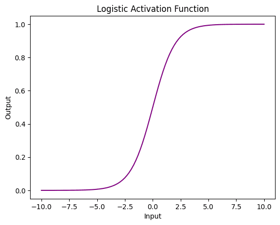
In the example above, you have used the torch.sigmoid() function from the Pytorch library to apply the logistic activation function to a tensor x. You have used the matplotlib library to create the plot with a custom color.
Tanh Activation Function
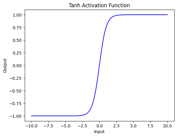
Next, you will investigate the tanh activation function which outputs values between $-1$ and $1$, with a mean output of 0. This can help ensure that the output of a neural network layer remains centered around 0, making it useful for normalization purposes. Tanh is a smooth and continuous activation function, which makes it easier to optimize during the process of gradient descent.
Like the logistic activation function, the tanh function can be susceptible to the vanishing gradient problem, especially for deep neural networks with many layers. This is because the slope of the function becomes very small for large or small input values, making it difficult for gradients to propagate through the network.
Also, due to the use of exponential functions, tanh can be computationally expensive, especially for large tensors or when used in deep neural networks with many layers.
Here is how to apply tanh on a tensor and visualize it.
|
1 2 3 4 5 6 7 8 9 |
# apply the tanh activation function to the tensor y = torch.tanh(x) # plot the results with a custom color plt.plot(x.numpy(), y.numpy(), color='blue') plt.xlabel('Input') plt.ylabel('Output') plt.title('Tanh Activation Function') plt.show() |
ReLU Activation Function
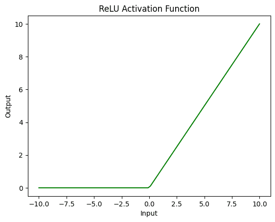
ReLU (Rectified Linear Unit) is another commonly used activation function in neural networks. Unlike the sigmoid and tanh functions, ReLU is a non-saturating function, which means that it does not become flat at the extremes of the input range. Instead, ReLU simply outputs the input value if it is positive, or 0 if it is negative.
This simple, piecewise linear function has several advantages over sigmoid and tanh activation functions. First, it is computationally more efficient, making it well-suited for large-scale neural networks. Second, ReLU has been shown to be less susceptible to the vanishing gradient problem, as it does not have a flattened slope. Plus, ReLU can help sparsify the activation of neurons in a network, which can lead to better generalization.
Here’s an example of how to apply the ReLU activation function to a PyTorch tensor x and plot the results.
|
1 2 3 4 5 6 7 8 9 |
# apply the ReLU activation function to the tensor y = torch.relu(x) # plot the results with a custom color plt.plot(x.numpy(), y.numpy(), color='green') plt.xlabel('Input') plt.ylabel('Output') plt.title('ReLU Activation Function') plt.show() |
Below is the complete code to print all the activation functions discussed above.
|
1 2 3 4 5 6 7 8 9 10 11 12 13 14 15 16 17 18 19 20 21 22 23 24 25 26 27 28 29 30 |
# importing the libraries import torch import matplotlib.pyplot as plt # create a PyTorch tensor x = torch.linspace(-10, 10, 100) # apply the logistic activation function to the tensor and plot y = torch.sigmoid(x) plt.plot(x.numpy(), y.numpy(), color='purple') plt.xlabel('Input') plt.ylabel('Output') plt.title('Logistic Activation Function') plt.show() # apply the tanh activation function to the tensor and plot y = torch.tanh(x) plt.plot(x.numpy(), y.numpy(), color='blue') plt.xlabel('Input') plt.ylabel('Output') plt.title('Tanh Activation Function') plt.show() # apply the ReLU activation function to the tensor and plot y = torch.relu(x) plt.plot(x.numpy(), y.numpy(), color='green') plt.xlabel('Input') plt.ylabel('Output') plt.title('ReLU Activation Function') plt.show() |
Exploring Activation Functions in a Neural Network
Activation functions play a vital role in the training of deep learning models, as they introduce non-linearity into the network, enabling it to learn complex patterns.
Let’s take the popular MNIST dataset, which consists of 70000 grayscale images in 28×28 pixels of handwritten digits. You’ll create a simple feedforward neural network to classify these digits, and experiment with different activation functions like ReLU, Sigmoid, Tanh, and Leaky ReLU.
|
1 2 3 4 5 6 7 8 9 10 11 |
import torchvision.datasets as datasets import torchvision.transforms as transforms from torch.utils.data import DataLoader # Load the MNIST dataset transform = transforms.ToTensor() train_dataset = datasets.MNIST(root='data/', train=True, transform=transform, download=True) test_dataset = datasets.MNIST(root='data/', train=False, transform=transform, download=True) train_loader = DataLoader(dataset=train_dataset, batch_size=64, shuffle=True) test_loader = DataLoader(dataset=test_dataset, batch_size=64, shuffle=False) |
Let’s create a NeuralNetwork class that inherits from nn.Module. This class has three linear layers and an activation function as an input parameter. The forward method defines the forward pass of the network, applying the activation function after each linear layer except the last one.
|
1 2 3 4 5 6 7 8 9 10 11 12 13 14 15 16 17 |
import torch import torch.nn as nn import torch.optim as optim class NeuralNetwork(nn.Module): def __init__(self, input_size, hidden_size, num_classes, activation_function): super(NeuralNetwork, self).__init__() self.layer1 = nn.Linear(input_size, hidden_size) self.layer2 = nn.Linear(hidden_size, hidden_size) self.layer3 = nn.Linear(hidden_size, num_classes) self.activation_function = activation_function def forward(self, x): x = self.activation_function(self.layer1(x)) x = self.activation_function(self.layer2(x)) x = self.layer3(x) return x |
You’ve added an activation_function parameter to the NeuralNetwork class, which allows you to plug in any activation function you’d like to experiment with.
Training and Testing the Model with Different Activation Functions
Let’s create functions to help the training. The train() function trains the network for one epoch. It iterates through the training data loader, computes the loss, and performs backpropagation and optimization. The test() function evaluates the network on the test dataset, computing the test loss and accuracy.
|
1 2 3 4 5 6 7 8 9 10 11 12 13 14 15 16 17 18 19 20 21 22 23 24 25 26 27 28 29 30 31 32 33 34 35 36 37 |
def train(network, data_loader, criterion, optimizer, device): network.train() running_loss = 0.0 for data, target in data_loader: data, target = data.to(device), target.to(device) data = data.view(data.shape[0], -1) optimizer.zero_grad() output = network(data) loss = criterion(output, target) loss.backward() optimizer.step() running_loss += loss.item() * data.size(0) return running_loss / len(data_loader.dataset) def test(network, data_loader, criterion, device): network.eval() correct = 0 total = 0 test_loss = 0.0 with torch.no_grad(): for data, target in data_loader: data, target = data.to(device), target.to(device) data = data.view(data.shape[0], -1) output = network(data) loss = criterion(output, target) test_loss += loss.item() * data.size(0) _, predicted = torch.max(output.data, 1) total += target.size(0) correct += (predicted == target).sum().item() return test_loss / len(data_loader.dataset), 100 * correct / total |
To compare them, let’s create a dictionary of activation functions and iterate over them. For each activation function, you instantiate the NeuralNetwork class, define the criterion (CrossEntropyLoss), and set up the optimizer (Adam). Then, train the model for a specified number of epochs, calling the train() and test() functions in each epoch to evaluate the model’s performance. You store the training loss, testing loss, and testing accuracy for each epoch in the results dictionary.
|
1 2 3 4 5 6 7 8 9 10 11 12 13 14 15 16 17 18 19 20 21 22 23 24 25 26 27 28 29 30 31 32 33 34 35 36 37 38 39 40 41 42 43 |
device = torch.device('cuda' if torch.cuda.is_available() else 'cpu') input_size = 784 hidden_size = 128 num_classes = 10 num_epochs = 10 learning_rate = 0.001 activation_functions = { 'ReLU': nn.ReLU(), 'Sigmoid': nn.Sigmoid(), 'Tanh': nn.Tanh(), 'LeakyReLU': nn.LeakyReLU() } results = {} # Train and test the model with different activation functions for name, activation_function in activation_functions.items(): print(f"Training with {name} activation function...") model = NeuralNetwork(input_size, hidden_size, num_classes, activation_function).to(device) criterion = nn.CrossEntropyLoss() optimizer = optim.Adam(model.parameters(), lr=learning_rate) train_loss_history = [] test_loss_history = [] test_accuracy_history = [] for epoch in range(num_epochs): train_loss = train(model, train_loader, criterion, optimizer, device) test_loss, test_accuracy = test(model, test_loader, criterion, device) train_loss_history.append(train_loss) test_loss_history.append(test_loss) test_accuracy_history.append(test_accuracy) print(f"Epoch [{epoch+1}/{num_epochs}], Test Loss: {test_loss:.4f}, Test Accuracy: {test_accuracy:.2f}%") results[name] = { 'train_loss_history': train_loss_history, 'test_loss_history': test_loss_history, 'test_accuracy_history': test_accuracy_history } |
When you run the above, it prints:
|
1 2 3 4 5 6 7 8 9 10 11 12 13 14 15 16 17 18 19 20 21 22 23 24 25 26 27 28 29 30 31 32 33 34 35 36 37 38 39 40 41 42 43 44 |
Training with ReLU activation function... Epoch [1/10], Test Loss: 0.1589, Test Accuracy: 95.02% Epoch [2/10], Test Loss: 0.1138, Test Accuracy: 96.52% Epoch [3/10], Test Loss: 0.0886, Test Accuracy: 97.15% Epoch [4/10], Test Loss: 0.0818, Test Accuracy: 97.50% Epoch [5/10], Test Loss: 0.0783, Test Accuracy: 97.47% Epoch [6/10], Test Loss: 0.0754, Test Accuracy: 97.80% Epoch [7/10], Test Loss: 0.0832, Test Accuracy: 97.56% Epoch [8/10], Test Loss: 0.0783, Test Accuracy: 97.78% Epoch [9/10], Test Loss: 0.0789, Test Accuracy: 97.75% Epoch [10/10], Test Loss: 0.0735, Test Accuracy: 97.99% Training with Sigmoid activation function... Epoch [1/10], Test Loss: 0.2420, Test Accuracy: 92.81% Epoch [2/10], Test Loss: 0.1718, Test Accuracy: 94.99% Epoch [3/10], Test Loss: 0.1339, Test Accuracy: 96.06% Epoch [4/10], Test Loss: 0.1141, Test Accuracy: 96.42% Epoch [5/10], Test Loss: 0.1004, Test Accuracy: 97.00% Epoch [6/10], Test Loss: 0.0909, Test Accuracy: 97.10% Epoch [7/10], Test Loss: 0.0846, Test Accuracy: 97.28% Epoch [8/10], Test Loss: 0.0797, Test Accuracy: 97.42% Epoch [9/10], Test Loss: 0.0785, Test Accuracy: 97.58% Epoch [10/10], Test Loss: 0.0795, Test Accuracy: 97.58% Training with Tanh activation function... Epoch [1/10], Test Loss: 0.1660, Test Accuracy: 95.17% Epoch [2/10], Test Loss: 0.1152, Test Accuracy: 96.47% Epoch [3/10], Test Loss: 0.1057, Test Accuracy: 96.86% Epoch [4/10], Test Loss: 0.0865, Test Accuracy: 97.21% Epoch [5/10], Test Loss: 0.0760, Test Accuracy: 97.61% Epoch [6/10], Test Loss: 0.0856, Test Accuracy: 97.23% Epoch [7/10], Test Loss: 0.0735, Test Accuracy: 97.66% Epoch [8/10], Test Loss: 0.0790, Test Accuracy: 97.67% Epoch [9/10], Test Loss: 0.0805, Test Accuracy: 97.47% Epoch [10/10], Test Loss: 0.0834, Test Accuracy: 97.82% Training with LeakyReLU activation function... Epoch [1/10], Test Loss: 0.1587, Test Accuracy: 95.14% Epoch [2/10], Test Loss: 0.1084, Test Accuracy: 96.37% Epoch [3/10], Test Loss: 0.0861, Test Accuracy: 97.22% Epoch [4/10], Test Loss: 0.0883, Test Accuracy: 97.06% Epoch [5/10], Test Loss: 0.0870, Test Accuracy: 97.37% Epoch [6/10], Test Loss: 0.0929, Test Accuracy: 97.26% Epoch [7/10], Test Loss: 0.0824, Test Accuracy: 97.54% Epoch [8/10], Test Loss: 0.0785, Test Accuracy: 97.77% Epoch [9/10], Test Loss: 0.0908, Test Accuracy: 97.92% Epoch [10/10], Test Loss: 0.1012, Test Accuracy: 97.76% |
You may use Matplotlib to create plots comparing the performance of each activation function. You can create three separate plots to visualize the training loss, testing loss, and testing accuracy for each activation function over the epochs.
|
1 2 3 4 5 6 7 8 9 10 11 12 13 14 15 16 17 18 19 20 21 22 23 24 25 26 27 28 |
import matplotlib.pyplot as plt # Plot the training loss plt.figure() for name, data in results.items(): plt.plot(data['train_loss_history'], label=name) plt.xlabel('Epoch') plt.ylabel('Training Loss') plt.legend() plt.show() # Plot the testing loss plt.figure() for name, data in results.items(): plt.plot(data['test_loss_history'], label=name) plt.xlabel('Epoch') plt.ylabel('Testing Loss') plt.legend() plt.show() # Plot the testing accuracy plt.figure() for name, data in results.items(): plt.plot(data['test_accuracy_history'], label=name) plt.xlabel('Epoch') plt.ylabel('Testing Accuracy') plt.legend() plt.show() |
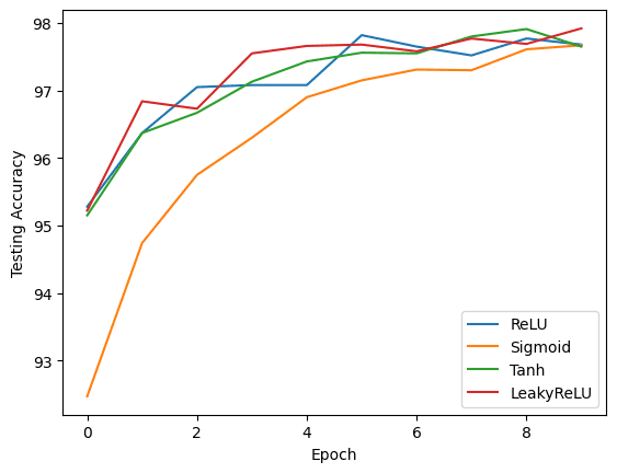
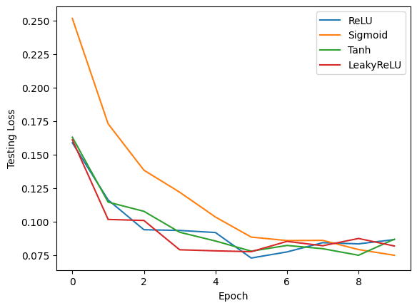
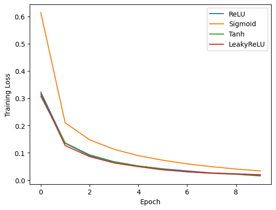
These plots provide a visual comparison of the performance of each activation function. By analyzing the results, you can determine which activation function works best for the specific task and dataset used in this example.
Summary
In this tutorial, you have implemented some of the most popular activation functions in PyTorch. You also saw how to train a neural network in PyTorch with different activation functions, using the popular MNIST dataset. You explored ReLU, Sigmoid, Tanh, and Leaky ReLU activation functions and analyzed their performance by plotting the training loss, testing loss, and testing accuracy.
As you can see, the choice of activation function plays an essential role in model performance. However, keep in mind that the optimal activation function may vary depending on the task and dataset.
Get Started on Deep Learning with PyTorch!

Learn how to build deep learning models
...using the newly released PyTorch 2.0 library
Discover how in my new Ebook:
Deep Learning with PyTorch
It provides self-study tutorials with hundreds of working code to turn you from a novice to expert. It equips you with
tensor operation, training, evaluation, hyperparameter optimization,
and much more...


Thank you for this tutorial. Can you please post something about sequence-to-sequence LSTM models in PyTorch as well?
You are very welcome Yeganekh! We appreciate the suggestion! The following may be of interest:
https://pytorch.org/tutorials/intermediate/seq2seq_translation_tutorial.html