
In this article, you will learn how LLM inference optimization works and which techniques to apply to make language models faster, cheaper, and more reliable in production.
Topics we will cover include:
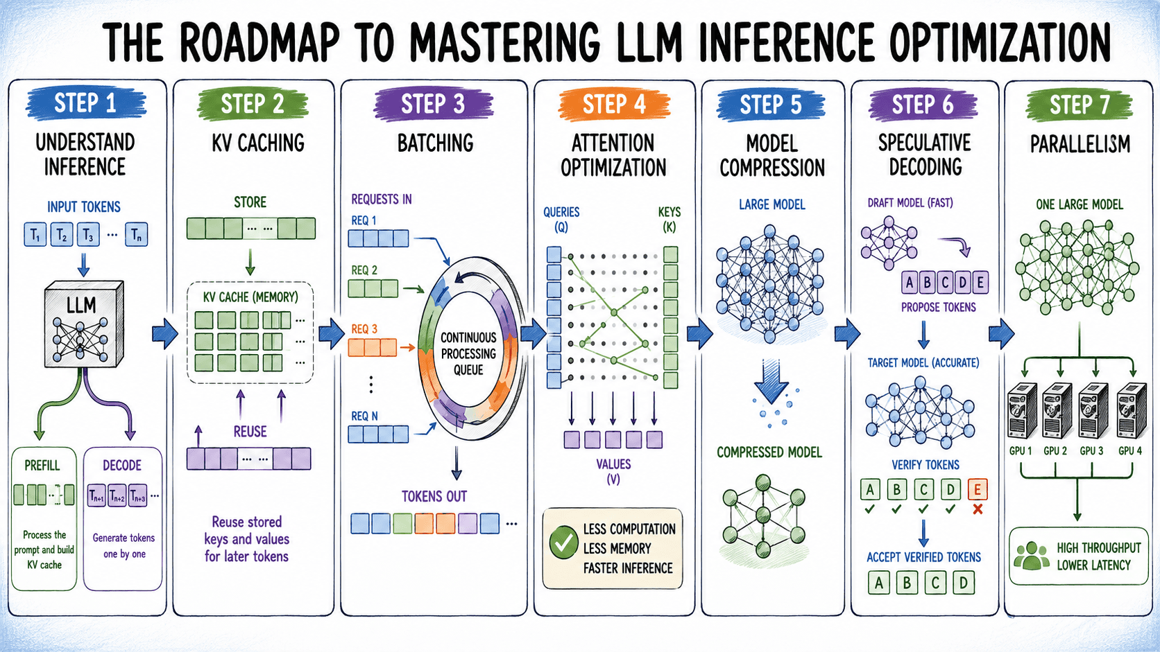
- How the two-phase inference process — prefill and decode — creates fundamentally different performance bottlenecks, and how understanding this distinction drives the choice of optimization technique.
- How memory management strategies like KV caching, PagedAttention, and prefix caching, combined with batching approaches and attention optimizations, directly improve throughput and latency.
- How model compression methods, speculative decoding, and multi-GPU parallelism can reduce inference cost and scale capacity for large or demanding workloads.
Let’s get straight into it.
Introduction
Getting a large language model to generate correct output is a solved problem for most teams. However, getting it to generate correct output fast enough, cheaply enough, and reliably enough in practice is where systems usually break down. A model may start missing latency targets the moment the request queue grows, and costs will scale faster than expected once batch sizes and context lengths increase.
Inference optimization is the discipline of closing that gap — the same model serves more requests, faster, at lower cost, without touching training. The techniques range from scheduling changes that require no model modifications at all to architecture-level attention variants baked into the model itself.
The place to start is understanding how LLM inference works.
Step 1: Understanding the Two-Phase Inference Process
Every forward pass through a decoder-only LLM involves two distinct phases with fundamentally different performance characteristics, and most optimization techniques target one or the other.
The first is the prefill phase. When a request arrives, the model processes all input tokens simultaneously to compute the intermediate states — the key and value tensors — needed to generate the first output token. Because the full input is known upfront, this computation is highly parallelized and saturates GPU utilization. Prefill is compute-bound.
The second is the decode phase. After the first output token is generated, the model produces subsequent tokens one at a time, autoregressively. Each new token depends on all previous tokens, which makes parallel generation within a single sequence impossible. The bottleneck here shifts: the GPU spends most of its time waiting for data to transfer from memory rather than on computation itself. Decode is memory-bandwidth-bound.
This distinction is important for everything that follows. GPU memory bandwidth, not raw compute, is the binding constraint during generation. Optimizations that reduce how much data the GPU has to move — or that let it do more useful work per memory access — directly translate to faster decoding.
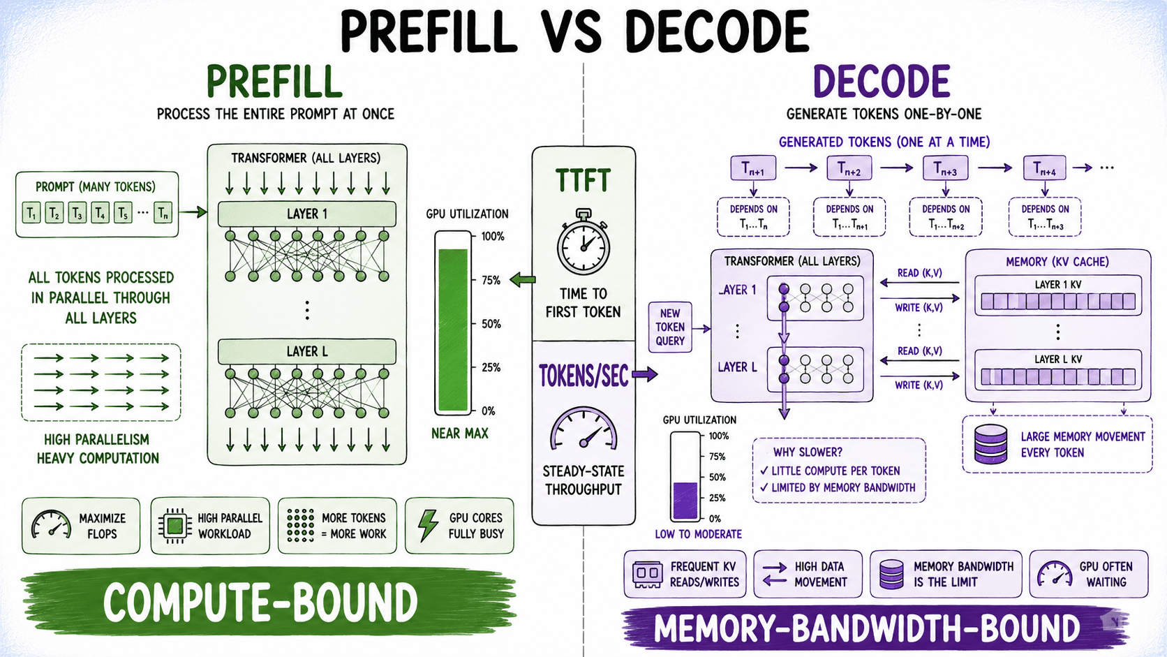
Understanding this also explains why simple benchmarks mislead. Time-to-first-token (TTFT) reflects prefill performance. Tokens per second (TPS) after the first token reflects decode performance. Optimizing one doesn’t necessarily improve the other, and the right technique depends on which metric your use case actually cares about.
To learn more, read From Prompt to Prediction: Understanding Prefill, Decode, and the KV Cache in LLMs.
Step 2: Understanding KV Caching and Why It Creates a Memory Problem
The most fundamental optimization for the decode phase is KV caching. Rather than recomputing key and value tensors for all previous tokens at every generation step, the model stores them in GPU memory and reuses them. This trades memory for compute — a good option when compute is expensive and memory is available.
The problem is that KV cache memory requirements scale with both batch size and sequence length simultaneously. For a 7B parameter model at 16-bit precision, the KV cache alone can consume several gigabytes per request at moderate sequence lengths. Scale up to long-context inputs or large batches and memory becomes the primary constraint on how many requests you can serve concurrently.
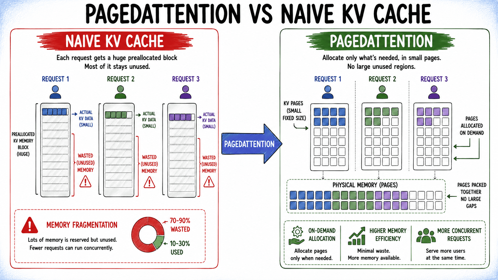
Naive KV cache management makes this worse. Allocating memory for the maximum possible sequence length upfront — because you can’t know in advance how long the generation will run — leads to significant internal fragmentation.
PagedAttention solves this by borrowing the virtual memory paging concept from operating systems. Instead of a single contiguous allocation per request, the KV cache is divided into fixed-size blocks that can be allocated non-contiguously and on demand as generation proceeds. New blocks are created as tokens are generated; nothing is pre-reserved. The result is dramatically lower memory waste, which directly enables larger batch sizes and higher throughput on the same hardware. vLLM implements this by default.
Prefix caching extends the idea further. When multiple requests share a common prefix — a system prompt, a document being analyzed, a few-shot example block — the KV cache for that prefix can be computed once and reused across all requests that share it. In RAG pipelines and applications with long system prompts, this can eliminate a significant fraction of redundant computation.
To learn more about how KV caching works and other inference caching techniques, check out KV Caching in LLMs: A Guide for Developers and The Complete Guide to Inference Caching in LLMs.
Step 3: Exploring Batching to Optimize GPU Utilization
A single request at a time leaves most of the GPU idle. The weights are loaded into memory for every forward pass regardless of how many tokens are being processed, so the amortized cost of those weights across the batch drops directly as batch size increases. Higher utilization means better throughput at lower per-token cost.
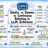
Static batching — waiting until a fixed batch is assembled before processing — is the naive implementation and it performs poorly in practice. Requests in a batch generate different numbers of output tokens. The batch can’t advance until the longest request finishes, which means faster requests idle while waiting. High variance in output length turns static batching into a significant throughput bottleneck.
Dynamic batching groups requests that arrive within a short time window, using a maximum batch size and timeout. The batch runs when either the maximum size is reached or the timeout expires, improving GPU utilization without making requests wait indefinitely. Shorter timeouts reduce latency but may create smaller batches, while longer timeouts can improve throughput at the cost of more queuing delay. However, once the batch starts, requests still progress together, so shorter requests can remain blocked by longer ones.
Continuous batching, also called in-flight batching, eliminates this by decoupling request completion from batch boundaries. As soon as a sequence finishes generating, it is evicted from the batch and a new request takes its slot — without waiting for other sequences in the batch to finish. The batch is continuously topped up rather than processed in fixed rounds. This keeps GPU utilization high even with highly variable output lengths and is now the default scheduling strategy in production runtimes like vLLM and TensorRT-LLM.
Read Static vs. Dynamic vs. Continuous Batching in LLM Inference for a more complete overview of these batching techniques.
Step 4: Optimizing the Attention Mechanism
Attention is the computationally dominant operation in most transformer forward passes, and it has accumulated several meaningful optimizations at the architecture level.
The standard multi-head attention (MHA) mechanism maintains separate key and value heads for each attention head. In multi-query attention (MQA), however, all query heads share a single set of key and value heads. The computation stays the same, but the amount of data that needs to move from memory during the decode phase drops substantially — which matters in a memory-bandwidth-bound operation. The tradeoff is a small accuracy regression, and models need to be trained or fine-tuned with MQA enabled to benefit from it at inference time.
Grouped-query attention (GQA) sits between MHA and MQA. Key and value heads are grouped, with multiple query heads sharing each group. You get most of MQA’s memory benefits while preserving more of MHA’s modeling capacity.
FlashAttention takes a different approach — it doesn’t change the attention architecture but changes how the computation is ordered. Standard attention implementations read and write intermediate values (the attention matrix) to GPU global memory repeatedly. FlashAttention fuses the attention operations and uses tiling to keep intermediate values in faster on-chip SRAM, dramatically reducing memory traffic without changing the mathematical output. It is a drop-in replacement for standard attention that requires no model retraining, which makes it one of the easiest optimizations to apply.
A Visual Guide to Attention Variants in Modern LLMs is an excellent resource for understanding some popular attention variants.
Step 5: Applying Model Compression
The techniques above improve how a model is served. Model compression reduces what needs to be served — making the model smaller and faster at a cost to precision that, when managed correctly, is smaller than you’d expect.
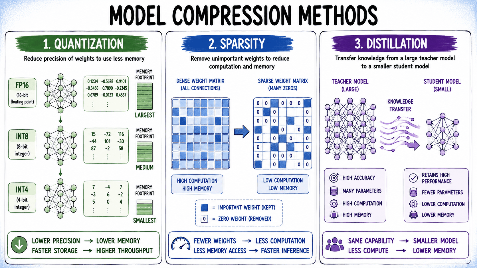
Quantization reduces the numerical precision of model weights and, optionally, activations. A model trained in 16-bit floating point takes roughly 2 bytes per parameter. At 8-bit integer precision, that drops to 1 byte; at 4-bit, 0.5 bytes. For a 7B parameter model, the difference between FP16 and INT4 is the gap between ~14 GB and ~3.5 GB of GPU memory — enough to change which hardware tier can serve the model at all. Quantization-aware techniques like GPTQ and AWQ have made 4-bit quantization of large models practical with minimal quality degradation, and GPUs have dedicated hardware for accelerating low-precision matrix operations.
Sparsity exploits the observation that many weight values in trained models are near zero and contribute minimally to outputs. Pruning these to exact zero creates sparse weight matrices that can be stored and computed more efficiently. NVIDIA’s Ampere and later GPU architectures include hardware support for 2:4 structured sparsity — where exactly two of every four values are zero — delivering up to 2x speedup on compatible operations with no additional software overhead.
Knowledge distillation trains a smaller student model to reproduce the behavior of a larger teacher model, rather than compressing the teacher directly. The student is trained on the teacher’s output distributions rather than ground-truth labels alone, which transfers more information than standard supervised training. For use cases where latency is the primary constraint, distillation often outperforms compression applied to the same original model because you’re starting with a better-matched architecture.
Step 6: Using Speculative Decoding for Latency-Critical Applications
The autoregressive constraint on token generation — each token must wait for the previous one — is the hardest bottleneck to break. Speculative decoding sidesteps it without violating the math.
The approach uses a small, fast draft model to generate a candidate sequence of several tokens. The full verification model then evaluates all of those tokens in parallel — which it can do because they’re treated as a batch of independent scoring problems rather than sequential generation steps. Tokens where the verification model agrees with the draft are accepted; the first disagreement causes everything after it to be discarded, and generation continues from that point.
The correctness guarantee is exact: accepted tokens are guaranteed to match what the full model would have generated on its own. The speed gain comes from the parallelized verification pass — when the draft model has high agreement with the full model, you effectively generate multiple tokens per full model call. The technique is most impactful in latency-sensitive, single-request scenarios where standard batching gains don’t apply, such as interactive chat. It provides less benefit in high-throughput batch workloads where batching already keeps the GPU busy.
The Machine Learning Practitioner’s Guide to Speculative Decoding is a useful reference.
Step 7: Scaling with Parallelism
When model size exceeds single-GPU memory capacity, or when throughput targets require more compute than one device can provide, parallelism distributes the load across multiple GPUs.
Tensor parallelism splits individual layers across devices. Weight matrices are partitioned so each GPU performs part of the computation, then devices synchronize the results. Its main benefit is reducing per-GPU weight memory while distributing computation for lower-latency inference.
Pipeline parallelism splits the model vertically, assigning consecutive layers to different GPUs. Each GPU processes its layers and passes activations to the next stage. Its main drawback is pipeline bubbles, where GPUs sit idle waiting for work. Microbatching reduces these bubbles by keeping multiple batches in flight. Pipeline parallelism is generally better suited to very large models and high-throughput workloads.
Prefill-decode disaggregation is a newer architectural pattern that routes prefill and decode phases to separate pools of hardware optimized for each. Prefill is compute-intensive and decode is memory-bandwidth-intensive — those are different hardware optimization targets. Disaggregating them lets each phase run on hardware matched to its bottleneck and prevents long prefill operations from blocking decode capacity. This is increasingly relevant as context lengths grow.
Summary
LLM inference optimization is a layered discipline. Here’s an overview of what we’ve discussed:
| Concept | Key Ideas |
|---|---|
| Two-phase inference process | Understand the two stages of inference: prefill (parallel, compute-bound, determines time-to-first-token) and decode (autoregressive, memory-bandwidth-bound, determines tokens/sec). This distinction explains where different optimizations apply. |
| KV caching & memory management | Learn how KV cache avoids recomputing attention states during decoding, why it becomes a memory bottleneck for long contexts, and how PagedAttention and prefix caching improve memory efficiency and reuse computation. |
| Batching | Improve GPU utilization with batching. Compare static batching (fixed batches, idle time due to variable output lengths) with continuous/in-flight batching, which dynamically replaces completed requests to maximize throughput. |
| Attention optimization | Reduce attention overhead using multi-query attention (MQA), grouped-query attention (GQA), and FlashAttention. These techniques reduce memory movement and accelerate attention computation during inference. |
| Model compression | Shrink the model and reduce inference cost using quantization, sparsity, and knowledge distillation, enabling faster inference and lower memory usage with minimal accuracy degradation. |
| Speculative decoding | Reduce latency by using a small draft model to generate candidate tokens and a larger model to verify them in parallel, allowing multiple tokens to be accepted per verification step without changing the final output. |
| Parallelism | Scale inference across multiple GPUs using tensor parallelism, pipeline parallelism, and prefill-decode disaggregation to support larger models and higher throughput while balancing memory and compute resources. |
The right combination depends on your latency targets, throughput requirements, context lengths, and hardware budget. Profile your actual workload against those constraints, and add techniques in order of impact.
The following resources are worth reading alongside this article:
Happy learning!





No comments yet.