Many computationally expensive tasks for machine learning can be made parallel by splitting the work across multiple CPU cores, referred to as multi-core processing.
Common machine learning tasks that can be made parallel include training models like ensembles of decision trees, evaluating models using resampling procedures like k-fold cross-validation, and tuning model hyperparameters, such as grid and random search.
Using multiple cores for common machine learning tasks can dramatically decrease the execution time as a factor of the number of cores available on your system. A common laptop and desktop computer may have 2, 4, or 8 cores. Larger server systems may have 32, 64, or more cores available, allowing machine learning tasks that take hours to be completed in minutes.
In this tutorial, you will discover how to configure scikit-learn for multi-core machine learning.
After completing this tutorial, you will know:
- How to train machine learning models using multiple cores.
- How to make the evaluation of machine learning models parallel.
- How to use multiple cores to tune machine learning model hyperparameters.
Let’s get started.

Multi-Core Machine Learning in Python With Scikit-Learn
Photo by ER Bauer, some rights reserved.
Tutorial Overview
This tutorial is divided into five parts; they are:
- Multi-Core Scikit-Learn
- Multi-Core Model Training
- Multi-Core Model Evaluation
- Multi-Core Hyperparameter Tuning
- Recommendations
Multi-Core Scikit-Learn
Machine learning can be computationally expensive.
There are three main centers of this computational cost; they are:
- Training machine learning models.
- Evaluating machine learning models.
- Hyperparameter tuning machine learning models.
Worse, these concerns compound.
For example, evaluating machine learning models using a resampling technique like k-fold cross-validation requires that the training process is repeated multiple times.
- Evaluation Requires Repeated Training
Tuning model hyperparameters compounds this further as it requires the evaluation procedure repeated for each combination of hyperparameters tested.
- Tuning Requires Repeated Evaluation
Most, if not all, modern computers have multi-core CPUs. This includes your workstation, your laptop, as well as larger servers.
You can configure your machine learning models to harness multiple cores of your computer, dramatically speeding up computationally expensive operations.
The scikit-learn Python machine learning library provides this capability via the n_jobs argument on key machine learning tasks, such as model training, model evaluation, and hyperparameter tuning.
This configuration argument allows you to specify the number of cores to use for the task. The default is None, which will use a single core. You can also specify a number of cores as an integer, such as 1 or 2. Finally, you can specify -1, in which case the task will use all of the cores available on your system.
- n_jobs: Specify the number of cores to use for key machine learning tasks.
Common values are:
- n_jobs=None: Use a single core or the default configured by your backend library.
- n_jobs=4: Use the specified number of cores, in this case 4.
- n_jobs=-1: Use all available cores.
What is a core?
A CPU may have multiple physical CPU cores, which is essentially like having multiple CPUs. Each core may also have hyper-threading, a technology that under many circumstances allows you to double the number of cores.
For example, my workstation has four physical cores, which are doubled to eight cores due to hyper-threading. Therefore, I can experiment with 1-8 cores or specify -1 to use all cores on my workstation.
Now that we are familiar with the scikit-learn library’s capability to support multi-core parallel processing for machine learning, let’s work through some examples.
You will get different timings for all of the examples in this tutorial; share your results in the comments. You may also need to change the number of cores to match the number of cores on your system.
Note: Yes, I am aware of the timeit API, but chose against it for this tutorial. We are not profiling the code examples per se; instead, I want you to focus on how and when to use the multi-core capabilities of scikit-learn and that they offer real benefits. I wanted the code examples to be clean and simple to read, even for beginners. I set it as an extension to update all examples to use the timeit API and get more accurate timings. Share your results in the comments.
Multi-Core Model Training
Many machine learning algorithms support multi-core training via an n_jobs argument when the model is defined.
This affects not just the training of the model, but also the use of the model when making predictions.
A popular example is the ensemble of decision trees, such as bagged decision trees, random forest, and gradient boosting.
In this section we will explore accelerating the training of a RandomForestClassifier model using multiple cores. We will use a synthetic classification task for our experiments.
In this case, we will define a random forest model with 500 trees and use a single core to train the model.
|
1 2 3 |
... # define the model model = RandomForestClassifier(n_estimators=500, n_jobs=1) |
We can record the time before and after the call to the train() function using the time() function. We can then subtract the start time from the end time and report the execution time in the number of seconds.
The complete example of evaluating the execution time of training a random forest model with a single core is listed below.
|
1 2 3 4 5 6 7 8 9 10 11 12 13 14 15 16 17 |
# example of timing the training of a random forest model on one core from time import time from sklearn.datasets import make_classification from sklearn.ensemble import RandomForestClassifier # define dataset X, y = make_classification(n_samples=10000, n_features=20, n_informative=15, n_redundant=5, random_state=3) # define the model model = RandomForestClassifier(n_estimators=500, n_jobs=1) # record current time start = time() # fit the model model.fit(X, y) # record current time end = time() # report execution time result = end - start print('%.3f seconds' % result) |
Running the example reports the time taken to train the model with a single core.
In this case, we can see that it takes about 10 seconds.
How long does it take on your system? Share your results in the comments below.
|
1 |
10.702 seconds |
We can now change the example to use all of the physical cores on the system, in this case, four.
|
1 2 3 |
... # define the model model = RandomForestClassifier(n_estimators=500, n_jobs=4) |
The complete example of multi-core training of the model with four cores is listed below.
|
1 2 3 4 5 6 7 8 9 10 11 12 13 14 15 16 17 |
# example of timing the training of a random forest model on 4 cores from time import time from sklearn.datasets import make_classification from sklearn.ensemble import RandomForestClassifier # define dataset X, y = make_classification(n_samples=10000, n_features=20, n_informative=15, n_redundant=5, random_state=3) # define the model model = RandomForestClassifier(n_estimators=500, n_jobs=4) # record current time start = time() # fit the model model.fit(X, y) # record current time end = time() # report execution time result = end - start print('%.3f seconds' % result) |
Running the example reports the time taken to train the model with a single core.
In this case, we can see that the speed of execution more than halved to about 3.151 seconds.
How long does it take on your system? Share your results in the comments below.
|
1 |
3.151 seconds |
We can now change the number of cores to eight to account for the hyper-threading supported by the four physical cores.
|
1 2 3 |
... # define the model model = RandomForestClassifier(n_estimators=500, n_jobs=8) |
We can achieve the same effect by setting n_jobs to -1 to automatically use all cores; for example:
|
1 2 3 |
... # define the model model = RandomForestClassifier(n_estimators=500, n_jobs=-1) |
We will stick to manually specifying the number of cores for now.
The complete example of multi-core training of the model with eight cores is listed below.
|
1 2 3 4 5 6 7 8 9 10 11 12 13 14 15 16 17 |
# example of timing the training of a random forest model on 8 cores from time import time from sklearn.datasets import make_classification from sklearn.ensemble import RandomForestClassifier # define dataset X, y = make_classification(n_samples=10000, n_features=20, n_informative=15, n_redundant=5, random_state=3) # define the model model = RandomForestClassifier(n_estimators=500, n_jobs=8) # record current time start = time() # fit the model model.fit(X, y) # record current time end = time() # report execution time result = end - start print('%.3f seconds' % result) |
Running the example reports the time taken to train the model with a single core.
In this case, we can see that we got another drop in execution speed from about 3.151 to about 2.521 by using all cores.
How long does it take on your system? Share your results in the comments below.
|
1 |
2.521 seconds |
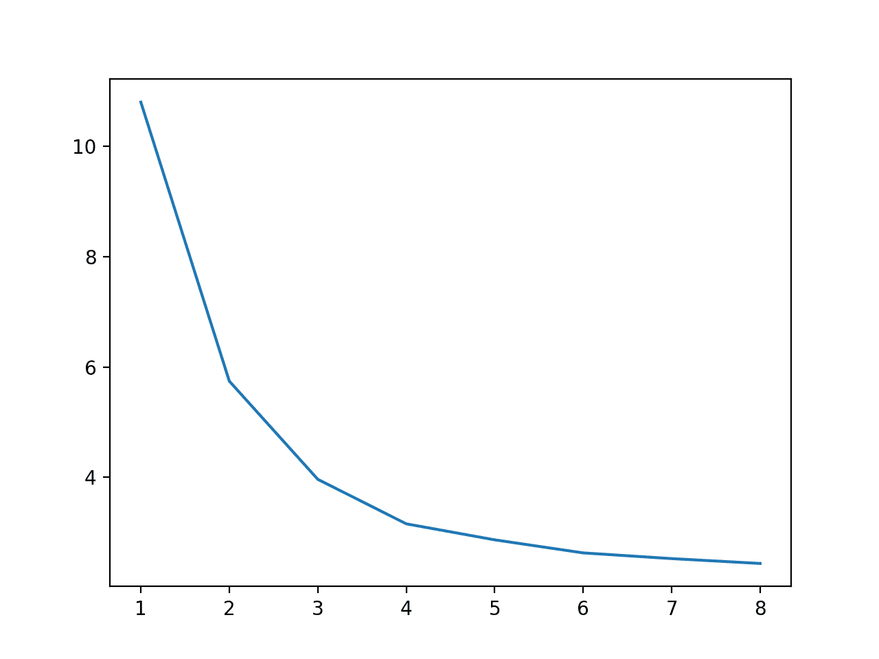
We can make the relationship between the number of cores used during training and execution speed more concrete by comparing all values between one and eight and plotting the result.
The complete example is listed below.
|
1 2 3 4 5 6 7 8 9 10 11 12 13 14 15 16 17 18 19 20 21 22 23 24 25 |
# example of comparing number of cores used during training to execution speed from time import time from sklearn.datasets import make_classification from sklearn.ensemble import RandomForestClassifier from matplotlib import pyplot # define dataset X, y = make_classification(n_samples=10000, n_features=20, n_informative=15, n_redundant=5, random_state=3) results = list() # compare timing for number of cores n_cores = [1, 2, 3, 4, 5, 6, 7, 8] for n in n_cores: # capture current time start = time() # define the model model = RandomForestClassifier(n_estimators=500, n_jobs=n) # fit the model model.fit(X, y) # capture current time end = time() # store execution time result = end - start print('>cores=%d: %.3f seconds' % (n, result)) results.append(result) pyplot.plot(n_cores, results) pyplot.show() |
Running the example first reports the execution speed for each number of cores used during training.
We can see a steady decrease in execution speed from one to eight cores, although the dramatic benefits stop after four physical cores.
How long does it take on your system? Share your results in the comments below.
|
1 2 3 4 5 6 7 8 |
>cores=1: 10.798 seconds >cores=2: 5.743 seconds >cores=3: 3.964 seconds >cores=4: 3.158 seconds >cores=5: 2.868 seconds >cores=6: 2.631 seconds >cores=7: 2.528 seconds >cores=8: 2.440 seconds |
A plot is also created to show the relationship between the number of cores used during training and the execution speed, showing that we continue to see a benefit all the way to eight cores.
Line Plot of Number of Cores Used During Training vs. Execution Speed
Now that we are familiar with the benefit of multi-core training of machine learning models, let’s look at multi-core model evaluation.
Multi-Core Model Evaluation
The gold standard for model evaluation is k-fold cross-validation.
This is a resampling procedure that requires that the model is trained and evaluated k times on different partitioned subsets of the dataset. The result is an estimate of the performance of a model when making predictions on data not used during training that can be used to compare and select a good or best model for a dataset.
In addition, it is also a good practice to repeat this evaluation process multiple times, referred to as repeated k-fold cross-validation.
The evaluation procedure can be configured to use multiple cores, where each model training and evaluation happens on a separate core. This can be done by setting the n_jobs argument on the call to cross_val_score() function; for example:
We can explore the effect of multiple cores on model evaluation.
First, let’s evaluate the model using a single core.
|
1 2 3 |
... # evaluate the model n_scores = cross_val_score(model, X, y, scoring='accuracy', cv=cv, n_jobs=1) |
We will evaluate the random forest model and use a single core in the training of the model (for now).
|
1 2 3 |
... # define the model model = RandomForestClassifier(n_estimators=100, n_jobs=1) |
The complete example is listed below.
|
1 2 3 4 5 6 7 8 9 10 11 12 13 14 15 16 17 18 19 20 21 |
# example of evaluating a model using a single core from time import time from sklearn.datasets import make_classification from sklearn.model_selection import cross_val_score from sklearn.model_selection import RepeatedStratifiedKFold from sklearn.ensemble import RandomForestClassifier # define dataset X, y = make_classification(n_samples=1000, n_features=20, n_informative=15, n_redundant=5, random_state=3) # define the model model = RandomForestClassifier(n_estimators=100, n_jobs=1) # define the evaluation procedure cv = RepeatedStratifiedKFold(n_splits=10, n_repeats=3, random_state=1) # record current time start = time() # evaluate the model n_scores = cross_val_score(model, X, y, scoring='accuracy', cv=cv, n_jobs=1) # record current time end = time() # report execution time result = end - start print('%.3f seconds' % result) |
Running the example evaluates the model using 10-fold cross-validation with three repeats.
In this case, we see that the evaluation of the model took about 6.412 seconds.
How long does it take on your system? Share your results in the comments below.
|
1 |
6.412 seconds |
We can update the example to use all eight cores of the system and expect a large speedup.
|
1 2 3 |
... # evaluate the model n_scores = cross_val_score(model, X, y, scoring='accuracy', cv=cv, n_jobs=8) |
The complete example is listed below.
|
1 2 3 4 5 6 7 8 9 10 11 12 13 14 15 16 17 18 19 20 21 |
# example of evaluating a model using 8 cores from time import time from sklearn.datasets import make_classification from sklearn.model_selection import cross_val_score from sklearn.model_selection import RepeatedStratifiedKFold from sklearn.ensemble import RandomForestClassifier # define dataset X, y = make_classification(n_samples=1000, n_features=20, n_informative=15, n_redundant=5, random_state=3) # define the model model = RandomForestClassifier(n_estimators=100, n_jobs=1) # define the evaluation procedure cv = RepeatedStratifiedKFold(n_splits=10, n_repeats=3, random_state=1) # record current time start = time() # evaluate the model n_scores = cross_val_score(model, X, y, scoring='accuracy', cv=cv, n_jobs=8) # record current time end = time() # report execution time result = end - start print('%.3f seconds' % result) |
Running the example evaluates the model using multiple cores.
In this case, we can see the execution timing dropped from 6.412 seconds to about 2.371 seconds, giving a welcome speedup.
How long does it take on your system? Share your results in the comments below.
|
1 |
2.371 seconds |
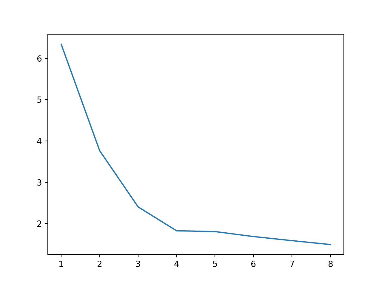
As we did in the previous section, we can time the execution speed for each number of cores from one to eight to get an idea of the relationship.
The complete example is listed below.
|
1 2 3 4 5 6 7 8 9 10 11 12 13 14 15 16 17 18 19 20 21 22 23 24 25 26 27 28 29 |
# compare execution speed for model evaluation vs number of cpu cores from time import time from sklearn.datasets import make_classification from sklearn.model_selection import cross_val_score from sklearn.model_selection import RepeatedStratifiedKFold from sklearn.ensemble import RandomForestClassifier from matplotlib import pyplot # define dataset X, y = make_classification(n_samples=1000, n_features=20, n_informative=15, n_redundant=5, random_state=3) results = list() # compare timing for number of cores n_cores = [1, 2, 3, 4, 5, 6, 7, 8] for n in n_cores: # define the model model = RandomForestClassifier(n_estimators=100, n_jobs=1) # define the evaluation procedure cv = RepeatedStratifiedKFold(n_splits=10, n_repeats=3, random_state=1) # record the current time start = time() # evaluate the model n_scores = cross_val_score(model, X, y, scoring='accuracy', cv=cv, n_jobs=n) # record the current time end = time() # store execution time result = end - start print('>cores=%d: %.3f seconds' % (n, result)) results.append(result) pyplot.plot(n_cores, results) pyplot.show() |
Running the example first reports the execution time in seconds for each number of cores for evaluating the model.
We can see that there is not a dramatic improvement above four physical cores.
We can also see a difference here when training with eight cores from the previous experiment. In this case, evaluating performance took 1.492 seconds whereas the standalone case took about 2.371 seconds.
This highlights the limitation of the evaluation methodology we are using where we are reporting the performance of a single run rather than repeated runs. There is some spin-up time required to load classes into memory and perform any JIT optimization.
Regardless of the accuracy of our flimsy profiling, we do see the familiar speedup of model evaluation with the increase of cores used during the process.
How long does it take on your system? Share your results in the comments below.
|
1 2 3 4 5 6 7 8 |
>cores=1: 6.339 seconds >cores=2: 3.765 seconds >cores=3: 2.404 seconds >cores=4: 1.826 seconds >cores=5: 1.806 seconds >cores=6: 1.686 seconds >cores=7: 1.587 seconds >cores=8: 1.492 seconds |
A plot of the relationship between the number of cores and the execution speed is also created.
Line Plot of Number of Cores Used During Evaluation vs. Execution Speed
We can also make the model training process parallel during the model evaluation procedure.
Although this is possible, should we?
To explore this question, let’s first consider the case where model training uses all cores and model evaluation uses a single core.
|
1 2 3 4 5 6 |
... # define the model model = RandomForestClassifier(n_estimators=100, n_jobs=8) ... # evaluate the model n_scores = cross_val_score(model, X, y, scoring='accuracy', cv=cv, n_jobs=1) |
The complete example is listed below.
|
1 2 3 4 5 6 7 8 9 10 11 12 13 14 15 16 17 18 19 20 21 |
# example of using multiple cores for model training but not model evaluation from time import time from sklearn.datasets import make_classification from sklearn.model_selection import cross_val_score from sklearn.model_selection import RepeatedStratifiedKFold from sklearn.ensemble import RandomForestClassifier # define dataset X, y = make_classification(n_samples=1000, n_features=20, n_informative=15, n_redundant=5, random_state=3) # define the model model = RandomForestClassifier(n_estimators=100, n_jobs=8) # define the evaluation procedure cv = RepeatedStratifiedKFold(n_splits=10, n_repeats=3, random_state=1) # record current time start = time() # evaluate the model n_scores = cross_val_score(model, X, y, scoring='accuracy', cv=cv, n_jobs=1) # record current time end = time() # report execution time result = end - start print('%.3f seconds' % result) |
Running the example evaluates the model using a single core, but each trained model uses a single core.
In this case, we can see that the model evaluation takes more than 10 seconds, much longer than the 1 or 2 seconds when we use a single core for training and all cores for parallel model evaluation.
How long does it take on your system? Share your results in the comments below.
|
1 |
10.461 seconds |
What if we split the number of cores between the training and evaluation procedures?
|
1 2 3 4 5 6 |
... # define the model model = RandomForestClassifier(n_estimators=100, n_jobs=4) ... # evaluate the model n_scores = cross_val_score(model, X, y, scoring='accuracy', cv=cv, n_jobs=4) |
The complete example is listed below.
|
1 2 3 4 5 6 7 8 9 10 11 12 13 14 15 16 17 18 19 20 21 |
# example of using multiple cores for model training and evaluation from time import time from sklearn.datasets import make_classification from sklearn.model_selection import cross_val_score from sklearn.model_selection import RepeatedStratifiedKFold from sklearn.ensemble import RandomForestClassifier # define dataset X, y = make_classification(n_samples=1000, n_features=20, n_informative=15, n_redundant=5, random_state=3) # define the model model = RandomForestClassifier(n_estimators=100, n_jobs=8) # define the evaluation procedure cv = RepeatedStratifiedKFold(n_splits=10, n_repeats=3, random_state=4) # record current time start = time() # evaluate the model n_scores = cross_val_score(model, X, y, scoring='accuracy', cv=cv, n_jobs=4) # record current time end = time() # report execution time result = end - start print('%.3f seconds' % result) |
Running the example evaluates the model using four cores, and each model is trained using four different cores.
We can see an improvement over training with all cores and evaluating with one core, but at least for this model on this dataset, it is more efficient to use all cores for model evaluation and a single core for model training.
How long does it take on your system? Share your results in the comments below.
|
1 |
3.434 seconds |
Multi-Core Hyperparameter Tuning
It is common to tune the hyperparameters of a machine learning model using a grid search or a random search.
The scikit-learn library provides these capabilities via the GridSearchCV and RandomizedSearchCV classes respectively.
Both of these search procedures can be made parallel by setting the n_jobs argument, assigning each hyperparameter configuration to a core for evaluation.
The model evaluation itself could also be multi-core, as we saw in the previous section, and the model training for a given evaluation can also be training as we saw in the second before that. Therefore, the stack of potentially multi-core processes is starting to get challenging to configure.
In this specific implementation, we can make the model training parallel, but we don’t have control over how each model hyperparameter and how each model evaluation is made multi-core. The documentation is not clear at the time of writing, but I would guess that each model evaluation using a single core hyperparameter configuration is split into jobs.
Let’s explore the benefits of performing model hyperparameter tuning using multiple cores.
First, let’s evaluate a grid of different configurations of the random forest algorithm using a single core.
|
1 2 3 |
... # define grid search search = GridSearchCV(model, grid, n_jobs=1, cv=cv) |
The complete example is listed below.
|
1 2 3 4 5 6 7 8 9 10 11 12 13 14 15 16 17 18 19 20 21 22 23 24 25 26 |
# example of tuning model hyperparameters with a single core from time import time from sklearn.datasets import make_classification from sklearn.model_selection import RepeatedStratifiedKFold from sklearn.ensemble import RandomForestClassifier from sklearn.model_selection import GridSearchCV # define dataset X, y = make_classification(n_samples=1000, n_features=20, n_informative=15, n_redundant=5, random_state=3) # define the model model = RandomForestClassifier(n_estimators=100, n_jobs=1) # define the evaluation procedure cv = RepeatedStratifiedKFold(n_splits=10, n_repeats=3, random_state=1) # define grid grid = dict() grid['max_features'] = [1, 2, 3, 4, 5] # define grid search search = GridSearchCV(model, grid, n_jobs=1, cv=cv) # record current time start = time() # perform search search.fit(X, y) # record current time end = time() # report execution time result = end - start print('%.3f seconds' % result) |
Running the example tests different values of the max_features configuration for random forest, where each configuration is evaluated using repeated k-fold cross-validation.
In this case, the grid search on a single core takes about 28.838 seconds.
How long does it take on your system? Share your results in the comments below.
|
1 |
28.838 seconds |
We can now configure the grid search to use all available cores on the system, in this case, eight cores.
|
1 2 3 |
... # define grid search search = GridSearchCV(model, grid, n_jobs=8, cv=cv) |
We can then evaluate how long this multi-core grids search takes to execute. The complete example is listed below.
|
1 2 3 4 5 6 7 8 9 10 11 12 13 14 15 16 17 18 19 20 21 22 23 24 25 26 |
# example of tuning model hyperparameters with 8 cores from time import time from sklearn.datasets import make_classification from sklearn.model_selection import RepeatedStratifiedKFold from sklearn.ensemble import RandomForestClassifier from sklearn.model_selection import GridSearchCV # define dataset X, y = make_classification(n_samples=1000, n_features=20, n_informative=15, n_redundant=5, random_state=3) # define the model model = RandomForestClassifier(n_estimators=100, n_jobs=1) # define the evaluation procedure cv = RepeatedStratifiedKFold(n_splits=10, n_repeats=3, random_state=1) # define grid grid = dict() grid['max_features'] = [1, 2, 3, 4, 5] # define grid search search = GridSearchCV(model, grid, n_jobs=8, cv=cv) # record current time start = time() # perform search search.fit(X, y) # record current time end = time() # report execution time result = end - start print('%.3f seconds' % result) |
Running the example reports execution time for the grid search.
In this case, we see a factor of about four speed up from roughly 28.838 seconds to around 7.418 seconds.
How long does it take on your system? Share your results in the comments below.
|
1 |
7.418 seconds |
Intuitively, we would expect that making the grid search multi-core should be the focus and not model training.
Nevertheless, we can divide the number of cores between model training and the grid search to see if it offers a benefit for this model on this dataset.
|
1 2 3 4 5 6 |
... # define the model model = RandomForestClassifier(n_estimators=100, n_jobs=4) ... # define grid search search = GridSearchCV(model, grid, n_jobs=4, cv=cv) |
The complete example of multi-core model training and multi-core hyperparameter tuning is listed below.
|
1 2 3 4 5 6 7 8 9 10 11 12 13 14 15 16 17 18 19 20 21 22 23 24 25 26 |
# example of multi-core model training and hyperparameter tuning from time import time from sklearn.datasets import make_classification from sklearn.model_selection import RepeatedStratifiedKFold from sklearn.ensemble import RandomForestClassifier from sklearn.model_selection import GridSearchCV # define dataset X, y = make_classification(n_samples=1000, n_features=20, n_informative=15, n_redundant=5, random_state=3) # define the model model = RandomForestClassifier(n_estimators=100, n_jobs=4) # define the evaluation procedure cv = RepeatedStratifiedKFold(n_splits=10, n_repeats=3, random_state=1) # define grid grid = dict() grid['max_features'] = [1, 2, 3, 4, 5] # define grid search search = GridSearchCV(model, grid, n_jobs=4, cv=cv) # record current time start = time() # perform search search.fit(X, y) # record current time end = time() # report execution time result = end - start print('%.3f seconds' % result) |
In this case, we do see a decrease in execution speed compared to a single core case, but not as much benefit as assigning all cores to the grid search process.
How long does it take on your system? Share your results in the comments below.
|
1 |
14.148 seconds |
Recommendations
This section lists some general recommendations when using multiple cores for machine learning.
- Confirm the number of cores available on your system.
- Consider using an AWS EC2 instance with many cores to get an immediate speed up.
- Check the API documentation to see if the model/s you are using support multi-core training.
- Confirm multi-core training offers a measurable benefit on your system.
- When using k-fold cross-validation, it is probably better to assign cores to the resampling procedure and leave model training single core.
- When using hyperparamter tuning, it is probably better to make the search multi-core and leave the model training and evaluation single core.
Do you have any recommendations of your own?
Further Reading
This section provides more resources on the topic if you are looking to go deeper.
Related Tutorials
APIs
- How to optimize for speed, scikit-learn Documentation.
- Joblib: running Python functions as pipeline jobs
- timeit API.
- sklearn.ensemble.RandomForestClassifier API.
- sklearn.model_selection.cross_val_score API.
- sklearn.model_selection.GridSearchCV API.
- sklearn.model_selection.RandomizedSearchCV API.
- n_jobs scikit-learn argument.
Articles
Summary
In this tutorial, you discovered how to configure scikit-learn for multi-core machine learning.
Specifically, you learned:
- How to train machine learning models using multiple cores.
- How to make the evaluation of machine learning models parallel.
- How to use multiple cores to tune machine learning model hyperparameters.
Do you have any questions?
Ask your questions in the comments below and I will do my best to answer.
Discover Fast Machine Learning in Python!

Develop Your Own Models in Minutes
...with just a few lines of scikit-learn code
Learn how in my new Ebook:
Machine Learning Mastery With Python
Covers self-study tutorials and end-to-end projects like:
Loading data, visualization, modeling, tuning, and much more...
Finally Bring Machine Learning To
Your Own Projects
Skip the Academics. Just Results.


Hi Jason, thank you for the tutorial. I ran the examples on my new laptop Lenovo Yoga Slim 7 (https://www.tomshardware.com/news/lenovo-yoga-slim-7-review-tested)
Here are the results for comparison:
Jason’s workstation vs. Oliver’s laptop
—————————————————
Test 1: 10.702 seconds vs. 11.967 seconds
Test 2: 3.151 seconds vs. 3.287 seconds
Test 3: 2.521 seconds vs. 1.965 seconds
Test 4:
>cores=1: 10.798 seconds vs. 11.933 seconds
>cores=2: 5.743 seconds vs. 6.292 seconds
>cores=3: 3.964 seconds vs. 4.290 seconds
>cores=4: 3.158 seconds vs. 3.467 seconds
>cores=5: 2.868 seconds vs. 3.014 seconds
>cores=6: 2.631 seconds vs. 2.669 seconds
>cores=7: 2.528 seconds vs. 2.448 seconds
>cores=8: 2.440 seconds vs. 2.189 seconds
Test 5: 6.412 seconds vs. 6.451 seconds
Test 6: 2.371 seconds vs. 1.179 seconds
Test 7:
>cores=1: 6.339 seconds vs. 6.443 seconds
>cores=2: 3.765 seconds vs. 4.238 seconds
>cores=3: 2.404 seconds vs. 3.061 seconds
>cores=4: 1.826 seconds vs. 2.128 seconds
>cores=5: 1.806 seconds vs. 2.526 seconds
>cores=6: 1.686 seconds vs. 1.663 seconds
>cores=7: 1.587 seconds vs. 1.487 seconds
>cores=8: 1.492 seconds vs. 1.482 seconds
Test 8: 10.461 seconds vs. 3.263 seconds (can this be right?)
Test 9: 3.434 seconds vs. 1.395 seconds
Test 10: 28.838 seconds vs. 28.937 seconds
Test 11: 7.418 seconds vs. 5.033 seconds
Test 12: 14.148 seconds vs. 8.051 seconds
Cheers
Oliver
Nice work, thanks for sharing!
Has anyone compiled a Python ML program into a .exe thats uses mutiple cores for say hyper tuning and got around the problem of the exe falling over ?
Maybe this will help:
https://machinelearningmastery.com/faq/single-faq/how-do-i-deploy-my-python-file-as-an-application
Thanks Jason I am using Pyinstaller but certainly in default mode it does not handle muti core processing, whether there are tricks or switches to enable this I have yet to discover
I don’t know sorry. Perhaps contact the author of the project directly.
It may be a mutl window problem I am using Tkinter.
“This may help me and anyone else
Add the line multiprocessing.freeze_support() to your code before creating your window. It’s documented here”
From stackoverflow
Thanks for sharing. What is Tkinter?
Tkinter is a GUI interface library for Python, allows GUI applications to be developed
Thanks.
Jason, I was going through and trying the tests on my computer – is the example of using multiple cores for model training and evaluation where
# define the model
model = RandomForestClassifier(n_estimators=100, n_jobs=4)
# evaluate the model
n_scores = cross_val_score(model, X, y, scoring=’accuracy’, cv=cv, n_jobs=4)
In the main code block below it, It looks like you used n_jobs for n_scores = 8?
Thanks,
Dana
Yes, the text above the code says we are using 8.
You can change it to anything you like.
Wow nice blog I loved it but I want to know whether n_jobs is a base class attribute or it is only specific to random forest classifier .
Thanks.
n_jobs is available to only those algorithms that support parallel training, like ensembles. Review the API for your chosen algorithm if you are unsure.
Great Blog!
Learnt many new things
Thanks!
Hi Jason, thank you for the tutorial. I ran the examples on my laptop dell core i7 U5500 with 2 core 4 thread
Test 1: 16.842 seconds
Well done!
Hi Jason,
Just performed random test for testing purpose
>cores=1: 34.046 seconds
>cores=2: 20.409 seconds
>cores=3: 14.541 seconds
>cores=4: 11.483 seconds
>cores=5: 9.330 seconds
>cores=6: 8.326 seconds
>cores=7: 7.281 seconds
>cores=8: 6.996 seconds
>cores=10: 6.626 seconds
>cores=19: 6.336 seconds
>cores=100: 6.565 seconds
import multiprocessing as mp
print(“Number of Laptop Logical processors: “, mp.cpu_count())
Number of Laptop Logical processors: 8
Why giving processors more then 8 in list reduces time by
6.996 – 6.626,
0.3700000000000001 seconds
other numbers in list 19,100 are just random number …to see effect
Point No. 2 :- We can also use multiprocessing pool & other functions provided in multiprocessing to parallelize execution.
Very cool!
can we use multi core with TPOT
I think TPOT uses multicore already.
Is multi core only for few Scikit-Learn algorithms like Random forest or all algorithims
Only for algorithms that support training in parallel. It’s not all algorithms.
Thank you so much Jason for this extremely useful tutorial.
Adding this one simple parameter njobs=-1 has dropped the time taken from 24.67 sec to 4.76 sec for my RandomForestClassifier()
This is going to make a huge difference to the overall execution times for my ensembles.
Well done!
Dear Dr Jason,
I wish to report my experiments with n_jobs. In (1) refer to the simple n_jobs = 1 and n_jobs = 8 , for model and evaluation then (2) n_jobs = 1 for model and varying the number of cores, and n_jobs = 8 for model and varying the number of cores.
For (2), the behaviour is not what I expected.
Now:
(1) In the first half of this tutorial, I had all permutations of n_jobs = 1 and n_jobs 8 each for model and the cv.
From the above, time reduction occurs when the cross_val_score’s n_jobs=8. Increasing the n_jobs for model to 8 reduces performance slightly.
(2) Varying the number of cores for cvs, when n_jobs for models = 1 and 8.
When n_jobs = 1 or 8 for model’s n_jobs, there is an ‘erratic’ downward trend. This ‘erratic’ change cannot be explained. Nevertheless, when model’s n_jobs=8, the time increases.
Overall, if the model’s n_jobs increases, does not necessarily improve the execution speed. It increases the execution speed slightly. BUT for (2) it be explained why there is no constant decrease in execution speed.
Thank you,
Anthony of Sydney
Nice work.
Yes, we can expect some stochastic variance. Compare average and stdev rather than single runs – a mantra for most things on computers.
Dear Dr Jason,
In the last example using the grid search, I did an ‘all-in-one’ script where I commented-out the appropriate.
The results in table:
Like the author’s result (Dr Jason’s), increasing the n_jobs for the model does not improve performance. It can also be seen that increasing the number of n_jobs for the model increases execution time.
In sum for all of the tutorial examples, increasing n_jobs for the cvs (repeatedstratifiedkfold) or grid search improves performance, but increasing n_jobs for model increases execution speed = decreases performance slightly.
Thank you,
Anthony of Sydney
However, when
The results are as follows
Dear Dr Jason,
Apologies. I did the following n_jobs for model and grid search respectively: (1,1), (4,4),(1,8) and (8,8). The conclusions are the same
The conclusion is the same. Increase n_jobs for grid search reduces execution time. Increasing n_jobs for the model increases execution time. Sharing the number of n_jobs equally does not improve the execution time.
Thank you,
Anthony of Sydney
Nice!
My computer :
AMD Ryzen 7 3700x (16 Threads) – 32GB. RAM @ 3600Mhz.
Windows 10 & Linux (the tests were run under the windows env).
As I’ve 16 cores on my CPU, I’ve Pushed your scripts to … 16cores 🙂 for fun.
Test 1 multi cores : Multi-Core Model Training
#>cores=1: 11.458 seconds
#>cores=2: 5.885 seconds
#>cores=3: 4.104 seconds
#>cores=4: 3.203 seconds
#>cores=5: 2.676 seconds
#>cores=6: 2.260 seconds
#>cores=7: 1.978 seconds
#>cores=8: 1.805 seconds
#>cores=9: 1.709 seconds
#>cores=10: 1.585 seconds
#>cores=11: 1.531 seconds
#>cores=12: 1.457 seconds
#>cores=13: 1.419 seconds
#>cores=14: 1.359 seconds
#>cores=15: 1.317 seconds
#>cores=16: 1.302 seconds
Test 2 : Multi-Core Model Evaluation
#>cores=1: 6.084 seconds
#>cores=2: 3.786 seconds
#>cores=3: 2.717 seconds
#>cores=4: 2.301 seconds
#>cores=5: 1.907 seconds
#>cores=6: 1.723 seconds
#>cores=7: 1.091 seconds
#>cores=8: 0.973 seconds
#>cores=9: 1.678 seconds !!!! very strange …. I ‘ve tested numerous times, and the restults are confirmed.
#>cores=10: 0.969 seconds
#>cores=11: 0.848 seconds
#>cores=12: 0.843 seconds
#>cores=13: 0.838 seconds
#>cores=14: 0.824 seconds
#>cores=15: 0.870 seconds
#>cores=16: 0.893 seconds
# example of tuning model hyperparameters with a single core
# 27.340sec
# example of tuning model hyperparameters with 8 cores
# 5.090 seconds
# example of multi-core model training and hyperparameter tuning
# 6.295 seconds
If I push to 8 jobs, The execution time is as low as 4.5 secs.
# example of multi-core model training and hyperparameter tuning
# 6.491 seconds … much quicker than your computer … this is strange
Finally, On one core your computer look quicker than mine on training, but slower on evaluation 🙂
There is also a strage phenomenon when running 9 cores on my Computer – the performances are worse than for 8 cores.
The Final tests on “multi-core model training and hyperparameter tuning” look much improved performance on my side compare to your results. I cannot explain such differences with the same code, and previous results.
cheers Gilles
Nice work!
We might be seeing stochastic effects.
We might also start seeing overhead and other effects related to python JIT/memory management, etc.
Repeating experiments and taking the average might help.
I totally agree 🙂
I was thinking @ running numerous times the same code in order to get a better view (using average and/or graphics plots).
In fact I did it, but did not aggregate the results.
I was also thinking at graphing the results in term of acceleration versus one core.
For example :
I do not know how to insert a graphic here… But on my computer, it is obvious that spread between what we could imagine to get is much lower with what we observe.
Gilles
Nice!
Hi Jason,
I spent a bit of time this afternoon and I’ve modified your code in order to run multiple times the tests, and finally graph the whisker plots.
I choose 10 runs, but it is easily parametrable in the code.
It is really interresting, because the first run is always slower than the others.
on my whiskers plots the outlier is always the first run. I suspect that python keeps something in memory.
The other interresting thing is that there is almost no gain between 10 and 14 threads, but 15 and 16 threads improve notably the performance. From 0.8sec down to 0.6sec.
Enjoy 🙂
The same methodology can be used on all your codes for those who want to dig and get around the stochastic variance
here is the code:
Well done.
Yes, the first run has to boot up the python run time. Often when benchmarking we have to do a warm start and discard the first few runs.
Sorry the code did not indent correctly when copy/pasting
No problem, I added pre tags.
Hi Jason, This is a great article. Thanks for writing about multi-core processing so explicitly. I do parallel computing most of the time for my deep machine learning work. Just want to add two suggestions which I figured out while teaching parallel computing to my students :
1. Add one more parameter other than ‘njobs’ which is ‘verbose’ which enables us to print some comments regarding where the process is currently while using multiple cores. This helps to understand the backend process.
2. In windows, for using multiple cores, we need some additional setting which is this :
if __name__ == ‘__main__’:
Code with njobs=…
If we don’t provide this setting, then the evn though we provide more than one core, the job is processed on just one core.
Thanks for sharing!
Hi Jason .
With regards to the current topic of ‘multi-core-ml’ in python, can you suggest some ways to improve the speed of execution of a svm (sklearn.svm.SVC) binary classification model on 45K records , which is running for days ? I have tried the following code for distributed computing on spark , but to no benefit .
from sklearn.utils import parallel_backend
from joblibspark import register_spark
register_spark()
from sklearn.svm import SVC
svm = SVC(kernel = ‘linear’, probability = True , class_weight = ‘balanced’, random_state = 12 )
with parallel_backend(‘spark’, n_jobs = 4):
%time feature_selection(model = svm, data = train_data_3, cont_features = cont_features)
Thanks!
Perhaps these ideas will help:
https://machinelearningmastery.com/faq/single-faq/how-do-i-speed-up-the-training-of-my-model
Thanks Jason.
You’re welcome.
hello Jason,
I have a 2.2 GHz Quad-Core Intel Core i7 Macbook 2015 model
For the comparing number of cores code i got the below output. It seems pretty fast.
>cores=1: 15.357 seconds
>cores=2: 8.948 seconds
>cores=3: 6.525 seconds
>cores=4: 4.728 seconds
>cores=5: 4.615 seconds
>cores=6: 5.048 seconds
>cores=7: 3.799 seconds
>cores=8: 3.987 seconds
tuning model hyperparameters with a single core take the below time
39.653 seconds
I had a question on the GridSearchCV. I am traning a model to fit the MNIST dataset which has the dimension 7000×784. This takes almost 30 mins per fit. How can this sped up?
from sklearn.model_selection import GridSearchCV
param_grid = [{‘weights’: [“uniform”, “distance”], ‘n_neighbors’: [3, 4, 5]}]
knn_clf = KNeighborsClassifier()
grid_search = GridSearchCV(knn_clf, param_grid, cv=5, verbose=3)
grid_search.fit(X_train, y_train)
Nice work.
Some suggestions:
Perhaps use GPUs?
Perhaps use more CPUs?
Perhaps use faster GPUs/CPUs?
Perhaps use a smaller model?
Perhaps use less data?
Perhaps use fewer hyperparameters in the search?
Hello Jason, thank you for your update on this multi-core process. I have a question on this. Can I enable multi-core calculation in RNN? I am using a sequential model and it seems that it doesn’t have a n_jobs argument.
Thank you for the reply.
Yes, Keras will use multiple CPU cores automatically.
Hi Jason,
I was just pondering…despite the inherent stochastic fluctuations, the non-increasing (or even decreasing) performance seen by some our friends above might be explained by the multi-threading behavior. The parallelism efficiency deteriorates for some operations when the computer starts using hyper-threading instead of the physical cores. This might happen when choosing n_jobs=8 cores in a 4 cores CPU like yours.
Does that make any sense?
Thanks for the helpful article.
Yes, that could be the case.
It highlights why it is important to test, rather than assume a linear or super-linear speedup.
Hi great article. I have one question. Can I set n_jobs = -1 for model training, evaluation and Hyperparameter tuning?
Sure.
“…I would guess that each model evaluation using a single core hyperparameter configuration is split into jobs.”
From looking at the GridSearchCV code that handles this[1], it looks like each combination of hyperparameter set + training split gets its own task (e.g. 5 splits * 2 hyperparam sets = 10 tasks).
…Which makes me wonder how caching a transformer[2] in grid search works. If joblib kicks off tasks for “Fold 1, hyperparam set A” and “Fold 1, hyperparam set B” at the same time, there’s no cached result to use until one of those finishes. Seems like you might not get the benefit of caching there, depending on what order the tasks are run in.
[1] https://github.com/scikit-learn/scikit-learn/blob/2beed5584/sklearn/model_selection/_search.py#L795
[2] https://scikit-learn.org/stable/modules/compose.html#caching-transformers-avoid-repeated-computation
You’re right. After all, caching is not guarantee to be faster. Cache invalidation should take into account too!
hello Jason
My name is Danial.
I have many problems about my thesis.
please please please help me.
Hi Danial…We would love to help answer any questions you have regarding the content we produce.
A great starting point can be found here:
https://machinelearningmastery.com/start-here/
Hi Jason,
I have a query when we train a ML/DL model using multicore processing, how the weights are shared across cores and how the model is saved at the end of training?
Hi Yogeeshwari…The following may be of interest to you.
https://www.analyticsvidhya.com/blog/2021/04/train-machine-learning-models-using-cpu-multi-cores/
The suggested link DO NOT ANSWER the asked question!
Thanks for the link!
Hi Jason, How we can finetune/train a hugging face transformer model using multiprocessing in pytorch? I am training in my personal Laptop. So kindly help me.
We all have some home powerful home PC’s. Also some expensive powerful Nvidia GPU’s at least on the paper. Now im much disappointed how Nvidia is utilizing CUDA for deep learning also for all the other parallels processing in the system and not using CUDA in SLI what would make much sense for parallel processing (SLI for other tasks not working well at all). Basically u re limited to one card only !? So how do pros use parallel processing on multiple GPUs ? Have installed Nvidia Tool and driver in order to utilize CUDA wide system support just found out that Phyton and other Data mining software not using CUDA at all. I have try to ad support manually installing required libraries but no luck at all. We have a “racing car sitting in the system parked in “garage” doing absolute nothing instead.
Why buy expensive hardware if one don’t have benefit from it ? And your NNs and data mining software is running as fast your CPU’s allow only. One would say at the end use Cloud Instead (don’t need a Comp just terminal then).
Hi Steve…You raise some interesting points! Let us know if we can help answer any questions regarding our content.
Look at this:
https://towardsdatascience.com/10x-faster-parallel-python-without-python-multiprocessing-e5017c93cce1
Even on multicore 24 cores Xeon CPU workstation phyton is equaly slow as on desktop CPU i7-7700K. Im switching to MatLab coz i need solutions coded only once for all the versions i test, thats one thing and not every time like in phyton, the other i need results somewhat fast no slow. Im sure that some of you with PhD in IT department look different on that matter and topics, but i’m only end user (not developer) and as eingeneer interested in end solutions and results and not so much in how and what. My point of view is that developed software on performance hardware should work work out of the box “plug’n play” a like and end user should not fight with it in order to get performance out of it. Phyton is nice programming language for simple and fast solutions, but soon as you start to requre performance … then things and problems get in the way, that one like me can not solve easly if even then so.
Cheers.