Image Augmentation with Keras Preprocessing Layers and tf.image

When you work on a machine learning problem related to images, not only do you need to collect some images as training data, but you also need to employ augmentation to create variations in the image. It is especially true for more complex object recognition problems.

There are many ways for image augmentation. You may use some external libraries or write your own functions for that. There are some modules in TensorFlow and Keras for augmentation too.

In this post, you will discover how you can use the Keras preprocessing layer as well as the tf.image module in TensorFlow for image augmentation.

After reading this post, you will know:

• What are the Keras preprocessing layers, and how to use them
• What are the functions provided by the tf.image module for image augmentation
• How to use augmentation together with the tf.data dataset

Let’s get started.

Image augmentation with Keras preprocessing layers and tf.image.
Photo by Steven Kamenar. Some rights reserved.

Overview

This article is divided into five sections; they are:

• Getting Images
• Visualizing the Images
• Keras Preprocessing Layers
• Using tf.image API for Augmentation
• Using Preprocessing Layers in Neural Networks

Getting Images

Before you see how you can do augmentation, you need to get the images. Ultimately, you need the images to be represented as arrays, for example, in HxWx3 in 8-bit integers for the RGB pixel value. There are many ways to get the images. Some can be downloaded as a ZIP file. If you’re using TensorFlow, you may get some image datasets from the tensorflow_datasets library.

In this tutorial, you will use the citrus leaves images, which is a small dataset of less than 100MB. It can be downloaded from tensorflow_datasets as follows:

Running this code the first time will download the image dataset into your computer with the following output:

The function above returns the images as a tf.data dataset object and the metadata. This is a classification dataset. You can print the training labels with the following:

This prints:

If you run this code again at a later time, you will reuse the downloaded image. But the other way to load the downloaded images into a tf.data dataset is to use the image_dataset_from_directory() function.

As you can see from the screen output above, the dataset is downloaded into the directory ~/tensorflow_datasets. If you look at the directory, you see the directory structure as follows:

The directories are the labels, and the images are files stored under their corresponding directory. You can let the function to read the directory recursively into a dataset:

You may want to set batch_size=None if you do not want the dataset to be batched. Usually, you want the dataset to be batched for training a neural network model.

Visualizing the Images

It is important to visualize the augmentation result, so you can verify the augmentation result is what we want it to be. You can use matplotlib for this.

In matplotlib, you have the imshow() function to display an image. However, for the image to be displayed correctly, the image should be presented as an array of 8-bit unsigned integers (uint8).

Given that you have a dataset created using image_dataset_from_directory()You can get the first batch (of 32 images) and display a few of them using imshow(), as follows:

Here, you see a display of nine images in a grid, labeled with their corresponding classification label, using ds.class_names. The images should be converted to NumPy array in uint8 for display. This code displays an image like the following: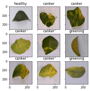

The complete code from loading the image to display is as follows:

Note that if you’re using tensorflow_datasets to get the image, the samples are presented as a dictionary instead of a tuple of (image,label). You should change your code slightly to the following:

For the rest of this post, assume the dataset is created using image_dataset_from_directory(). You may need to tweak the code slightly if your dataset is created differently.

Keras Preprocessing Layers

Keras comes with many neural network layers, such as convolution layers, that you need to train. There are also layers with no parameters to train, such as flatten layers to convert an array like an image into a vector.

The preprocessing layers in Keras are specifically designed to use in the early stages of a neural network. You can use them for image preprocessing, such as to resize or rotate the image or adjust the brightness and contrast. While the preprocessing layers are supposed to be part of a larger neural network, you can also use them as functions. Below is how you can use the resizing layer as a function to transform some images and display them side-by-side with the original:

The images are in 256×256 pixels, and the resizing layer will make them into 256×128 pixels. The output of the above code is as follows: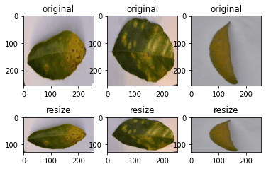

Since the resizing layer is a function, you can chain them to the dataset itself. For example,

The dataset ds has samples in the form of (image, label). Hence you created a function that takes in such tuple and preprocesses the image with the resizing layer. You then assigned this function as an argument for the map() in the dataset. When you draw a sample from the new dataset created with the map() function, the image will be a transformed one.

There are more preprocessing layers available. Some are demonstrated below.

As you saw above, you can resize the image. You can also randomly enlarge or shrink the height or width of an image. Similarly, you can zoom in or zoom out on an image. Below is an example of manipulating the image size in various ways for a maximum of 30% increase or decrease:

This code shows images as follows:

While you specified a fixed dimension in resize, you have a random amount of manipulation in other augmentations.

You can also do flipping, rotation, cropping, and geometric translation using preprocessing layers:

This code shows the following images: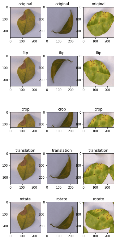

And finally, you can do augmentations on color adjustments as well:

This shows the images as follows: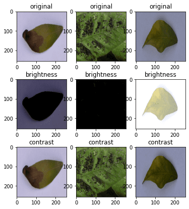

For completeness, below is the code to display the result of various augmentations:

Finally, it is important to point out that most neural network models can work better if the input images are scaled. While we usually use an 8-bit unsigned integer for the pixel values in an image (e.g., for display using imshow() as above), a neural network prefers the pixel values to be between 0 and 1 or between -1 and +1. This can be done with preprocessing layers too. Below is how you can update one of the examples above to add the scaling layer into the augmentation:

Using tf.image API for Augmentation

Besides the preprocessing layer, the tf.image module also provides some functions for augmentation. Unlike the preprocessing layer, these functions are intended to be used in a user-defined function and assigned to a dataset using map() as we saw above.

The functions provided by the tf.image are not duplicates of the preprocessing layers, although there is some overlap. Below is an example of using the tf.image functions to resize and crop images:

Below is the output of the above code:

While the display of images matches what you might expect from the code, the use of tf.image functions is quite different from that of the preprocessing layers. Every tf.image function is different. Therefore, you can see the crop_to_bounding_box() function takes pixel coordinates, but the central_crop() function assumes a fraction ratio as the argument.

These functions are also different in the way randomness is handled. Some of these functions do not assume random behavior. Therefore, the random resize should have the exact output size generated using a random number generator separately before calling the resize function. Some other functions, such as stateless_random_crop(), can do augmentation randomly, but a pair of random seeds in the int32 needs to be specified explicitly.

To continue the example, there are the functions for flipping an image and extracting the Sobel edges:

This shows the following: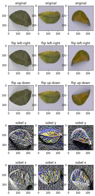

And the following are the functions to manipulate the brightness, contrast, and colors:

This code shows the following: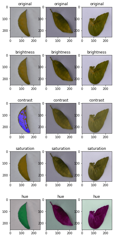

Below is the complete code to display all of the above:

These augmentation functions should be enough for most uses. But if you have some specific ideas on augmentation, you would probably need a better image processing library. OpenCV and Pillow are common but powerful libraries that allow you to transform images better.

Using Preprocessing Layers in Neural Networks

You used the Keras preprocessing layers as functions in the examples above. But they can also be used as layers in a neural network. It is trivial to use. Below is an example of how you can incorporate a preprocessing layer into a classification network and train it using a dataset:

Running this code gives the following output:

In the code above, you created the dataset with cache() and prefetch(). This is a performance technique to allow the dataset to prepare data asynchronously while the neural network is trained. This would be significant if the dataset has some other augmentation assigned using the map() function.

You will see some improvement in accuracy if you remove the RandomFlip and RandomRotation layers because you make the problem easier. However, as you want the network to predict well on a wide variation of image quality and properties, using augmentation can help your resulting network become more powerful.

Further Reading

Below is some documentation from TensorFlow that is related to the examples above:

• tf.data.Dataset API
• Citrus leaves dataset
• Load and preprocess images
• Data augmentation
• tf.image API
• tf.data performance

Summary

In this post, you have seen how you can use the tf.data dataset with image augmentation functions from Keras and TensorFlow.

Specifically, you learned:

• How to use the preprocessing layers from Keras, both as a function and as part of a neural network
• How to create your own image augmentation function and apply it to the dataset using the map() function
• How to use the functions provided by the tf.image module for image augmentation