By Luis Bermudez
This blog walks through a process for experimenting with hyperparameters, training algorithms and other parameters of Graph Neural Networks. In this post, we share the first two phases of our experiment chain. The graph datasets that we use to make inferences on come from Open Graph Benchmark (OGB). If you find it useful, we’ve provided a brief Overview of GNNs and a short Overview on OGB.
Experimentation Objectives and Model Types
We tuned two popular GNN variants to:
- Improve performance on OGB leaderboard prediction tasks.
- Minimize training cost (time and number of epochs) for future reference.
- Analyze mini-batch vs full graph training behavior across HPO iterations.
- Demonstrate a generic process for iterative experimentation on hyperparameters.
We made our own implementations of OGB leaderboard entries for two popular GNN frameworks: GraphSAGE and a Relational Graph Convolutional Network (RGCN). We then designed and executed an iterative experimentation approach for hyperparameter tuning where we seek a quality model that takes minimal time to train. We define quality by running an unconstrained performance tuning loop, and use the results to set thresholds in a constrained tuning loop that optimizes for training efficiency.
For GraphSAGE and RGCN we implemented both a mini batch and a full graph approach. Sampling is an important aspect of training GNNs, and the mini-batching process is different than when training other types of neural networks. In particular, mini-batching graphs can lead to exponential growth in the amount of data the network needs to process per batch – this is called “neighborhood explosion”. Below in the experiment design section, we describe our approach to tuning with this aspect of mini batching on graphs in mind.
To see more about the importance of sampling strategies for GNNs, check out some of these resources:
- Deep Graph Library (DGL) User Guide
- DGL Mini Batch Sampling API
- Accelerate Training and Inference of GNNs
- Mini Batch Sampling with GNNs
Now we seek to find the best versions of our models according to the experimentation objectives described above.
Iterative Experimentation: Optimizing for time to quality model
Our HPO (hyper parameter optimization) Experimentation process has three phases for each model type for both mini batch and full graph sampling. The three phases include:
- Performance: What is the best performance?
- Efficiency: How quickly can we find a quality model?
- Trust: How do we select the highest quality models?
The first phase leverages a single metric SigOpt Experiment that optimizes for validation loss for both mini batch and full graph implementations. This phase finds the best performance by tuning GraphSAGE and RCGN.
The second phase defines two metrics to measure how quickly we complete the model training: (a) wall clock time for GNN training, and (b) total epochs for GNN training. We also use our knowledge from the first phase to inform the design of a constrained optimization experiment. We minimize the metrics subject to the validation loss being greater than a quality target.
The third phase picks quality models with reasonable distance between them in hyperparameter space. We run the same training with 10 different random seeds per OGB guidelines. We also use the GNNExplainer to analyze the patterns across models. (We’ll elaborate more on the third phase in a future blog post)
How to run the code
The code lives in this repo. To run the code, you need to do these steps:
- Sign up for free or login to get your API Token
- Clone the repo
- Create virtual environment and run
|
1 2 3 4 5 6 7 8 9 10 11 12 13 14 15 16 17 18 19 20 |
# Place the API token as an environment variable > export SIGOPT_API_TOKEN=<> # Install the required libraries > pip install –r requirements.txt # Go to experiments/ and run > python create_experiment.py \ --model \ --dataset \ --training-method --optimization-target # Go to experiments/ and run > python run_experiment.py \ --experiment-id \ --model \ --dataset \ --training-method \ --optimization-target |

Phase 1 Results: Designing experiments to maximize accuracy
For the first phase of experimentation, the hyperparameter tuning Experiment was done on a Xeon cluster using Jenkins to schedule model training runs to cluster nodes. Docker containers were used for the execution environment. There were four streams of Experiments in total, one for each row in the following table, all aiming to minimize the validation loss.
| GNN Type | Dataset | Sampling | Optimization Target | Best Validation Loss | Best Validation Accuracy |
| GraphSAGE | ogbn-products | mini batch | Validation loss | 0.269 | 0.929 |
| GraphSAGE | ogbn-products | full graph | Validation loss | 0.306 | 0.92 |
| RGCN | ogbn-mag | mini batch | Validation loss | 1.781 | 0.506 |
| RGCN | ogbn-mag | full graph | Validation loss | 1.928 | 0.472 |
Table 1 – Results from Experiment Phase 1
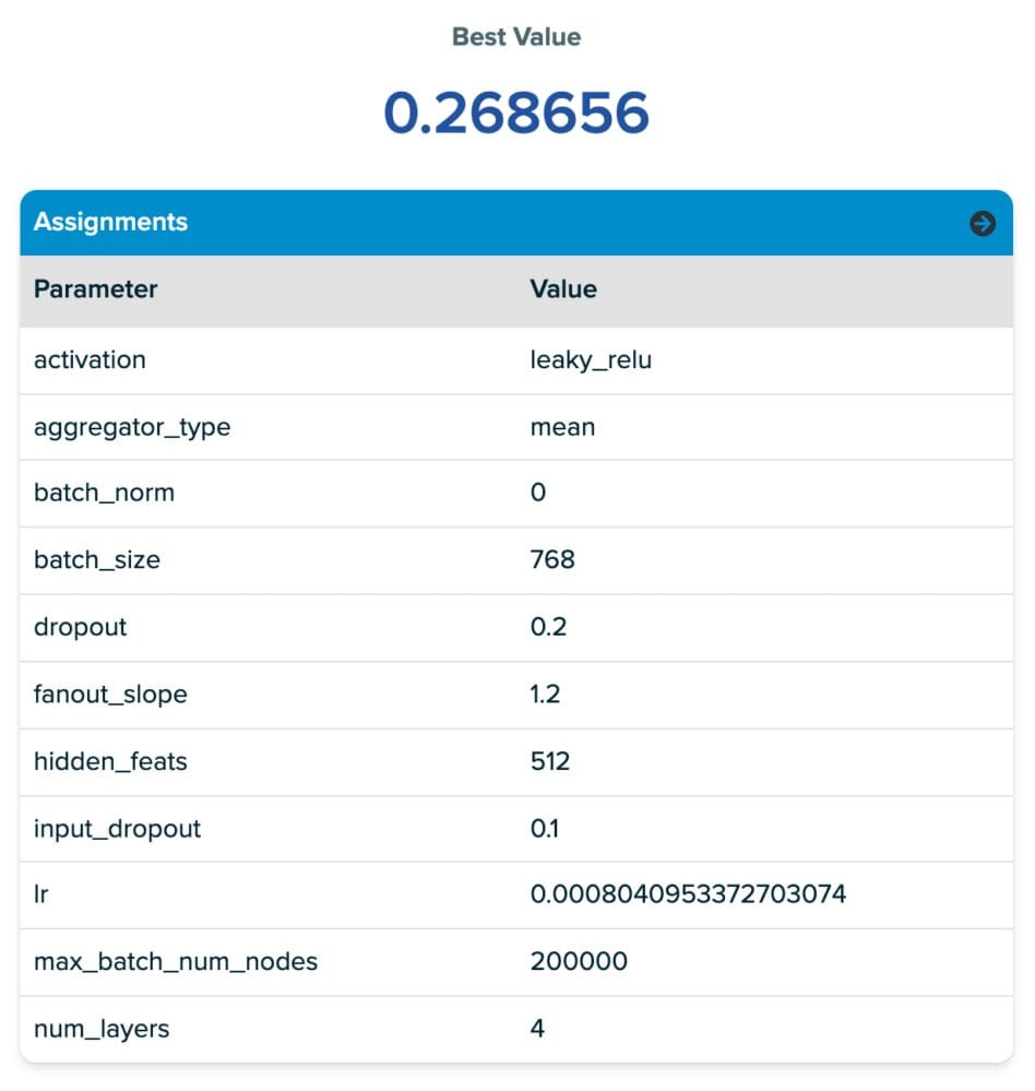
The parameter values for the first row in the table are provided in the screenshot of the SigOpt platform (right below the table). From the parameters screenshot, you will notice our tuning space contains many common neural network hyperparameters. You will also notice a few new ones called fanout slope and max_batch_num_nodes. These are both related to a parameter of Deep Graph Library MultiLayerNeighborSampler called fanouts which determines how many neighboring nodes are considered during message passing. We introduce these new parameters in the design space to encourage SigOpt to pick “good” fanouts from a reasonably large tuning space without directly tuning the number of fanouts, which we found often led to prohibitively long training times due to the neighborhood explosion when doing message passing through multiple layers of sampling. The objective with this approach is to explore the mini-batch sampling space while limiting the neighborhood explosion problem. The two parameters’ we introduce are:
- Fanout Slope: Controls rate of fanout per hop/GNN layer. Increasing it acts as a multiplier of the fanout, the number of nodes sampled in each additional hop in the graph.
- Max Batch Num Nodes: Sets a threshold for the maximum number of nodes per batch, if the total number of samples produced with fanout slope.
Below we see the RGCN Experiment configurations for phase 1. There is a similar deviation between mini batch and full graph implementations for our GraphSAGE Experiments.
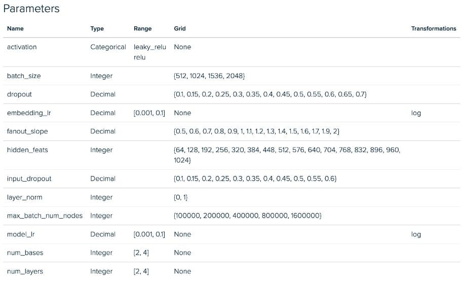
RGCN Mini Batch Tuning Experiment – Parameter Space
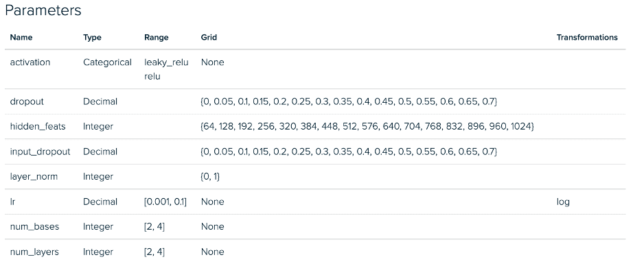
RGCN Full Graph Tuning Experiment – Parameter Space
Tuning GraphSAGE with a mini-batch approach we found that of the parameters we introduced, the fanout_slope was important in predicting accuracy scores and the max_batch_num_nodes were relatively unimportant. In particular, we found that the max_batch_num_nodes achieved tended to lead to points that performed better when it was low.
The results for the mini-batch RGCN showed something similar, although the max_batch_num_nodes parameters were slightly more impactful. Both mini-batch results showed better performance than their full-graph counterparts. All four hyperparameter tuning streams had the runs they contained early-stopping when performance did not improve after ten epochs.
This procedure yielded the following distributions:
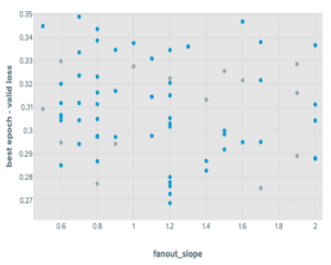
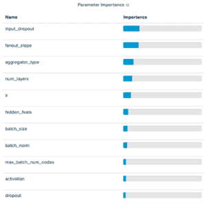
Results from Tuning Experiment of GraphSAGE on OGBN products
Next, we use the results from these experiments to inform the experiment design for a subsequent round focused on hitting a quality target as quickly as possible. For a quality target, we set a constraint at (1.05 * best validation loss) and (0.95 * accuracy score) for the validation loss and validation accuracy, respectively.
Phase 2 Results: Designing experiments for efficiency
During the second phase of experimentation, we seek models meeting our quality target that train as quickly as possible. We trained these models on Xeon processors on AWS m6.8xlarge instances. Our optimization task is to:
- Minimize total run time
- Subject to validation loss less than or equal to 1.05 times the best seen value
- Subject to validation accuracy greater than or equal to 0.95 times the best seen value
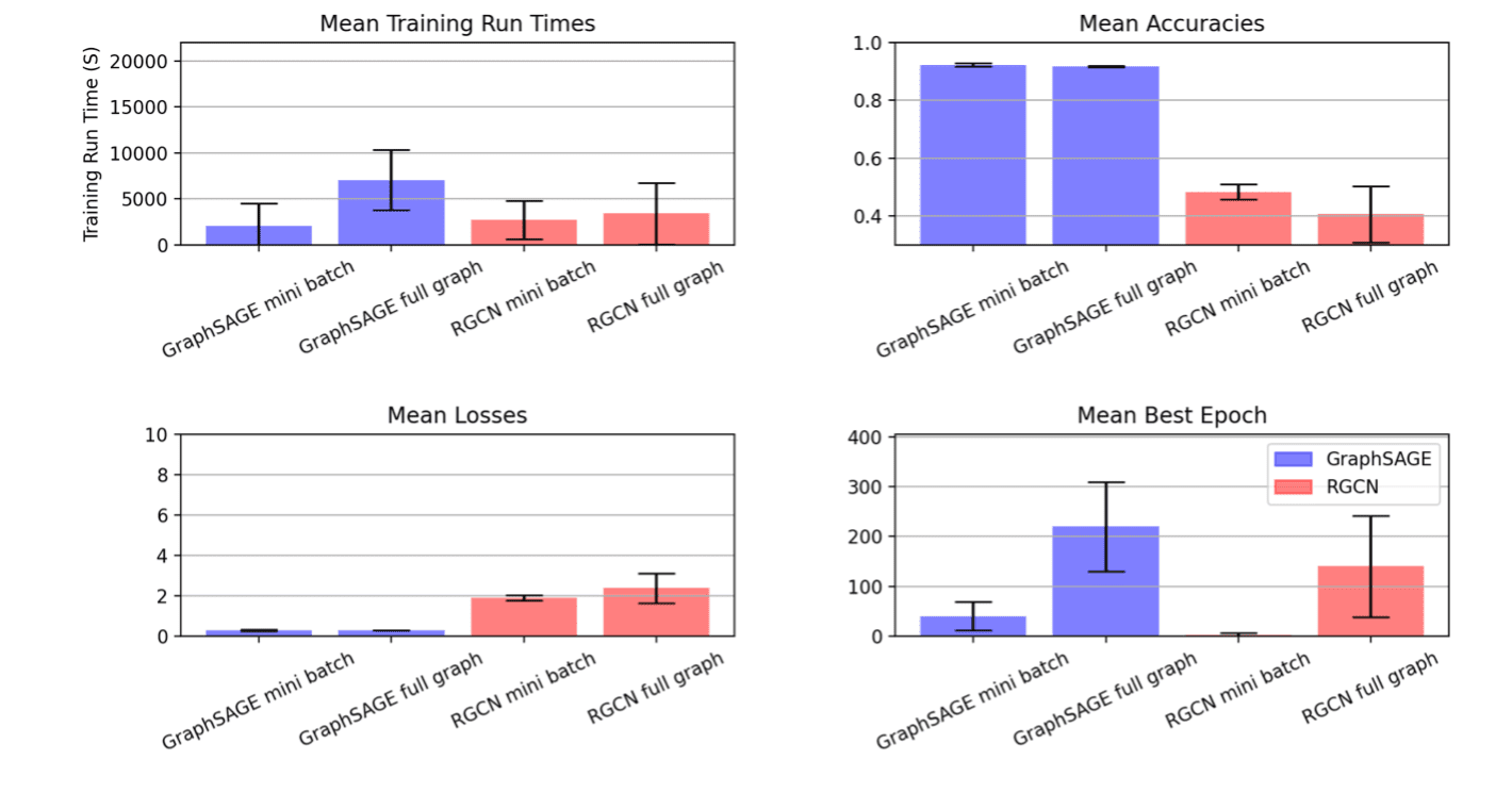
Framing our optimization targets in this way yielded these metric results
| GNN type | Dataset | Sampling | Optimization Target |
Best Time | Valid Accuracy |
| GraphSAGE | ogbn-products | mini batch | Training time, epochs | 933.529 | 0.929 |
| GraphSAGE | ogbn-products | full graph | Training time, epochs | 3791.15 | 0.923 |
| RGCN | ogbn-mag | mini batch | Training time, epochs | 155.321 | 0.515 |
| RGCN | ogbn-mag | full graph | Training time, epochs | 534.192 | 0.472 |
Note that this project was aiming to show the iterative experimentation process. The goal was not to keep everything constant besides the metric space between phase one and phase two, so we made adjustments to the tuning space for this second round of experiments. In the above plot, the result of this is visible in the RGCN mini batch runs where we see a large reduction in variance across runs after we significantly pruned the searchable hyperparameter domain based on analysis of the first phase of experiments.
Discussion
In the results, it is clear that the SigOpt optimizer is finding a lot of candidate runs that meet our performance thresholds while significantly reducing the amount of training time. Not only is this useful for this experimentation cycle, but insights derived from this extra work are likely to be reusable in future instances of workflows involving similar tuning jobs on GraphSAGE and RGCN being applied to OGBN-products and OGBN-mag, respectively. In a follow-up post, we will look at phase three of this process. We will select a few high-quality, low run-time model configurations and we will see how using state-of-the-art interpretability tools like GNNExplainer can facilitate further insight into how to select the right models.
To see if SigOpt can drive similar results for you and your team, sign up to use it for free.
This blog post was originally published on sigopt.com.



No comments yet.