When you are working on a data science project, the data is often tabular structured. You can use the built-in data table to handle such data in R. You can also use the famous library dplyr instead to benefit from its rich toolset. In this post, you will learn how dplyr can help you explore and manipulate tabular data. In particular, you will learn:
- How to handle a data frame
- How to perform some common operations on a data frame
Let’s get started.

Exploring Data using dplyr in R.
Photo by Airam Dato-on. Some rights reserved.
Overview
This post is divided into two parts; they are:
- Starting wih dplyr
- Exploring a dataset
Starting with dplyr
The library dplyr in R can be installed using the command install.package("dplyr") in R command line. But it is usually helpful to install the tidyverse package as it is a collection of some useful packages for data science:
|
1 |
install.package("tidyverse") |
Before you start, you should load the dplyr package, which will override some existing R functions and add new features:
|
1 |
library(dplyr) |
The dplyr library is a powerful data manipulation library. This library operates on tabular structured data called data frame. To create a data frame from scratch, you can use the following syntax:
|
1 2 3 4 5 |
df <- data.frame( name = c("Alice", "Bob", "Charlie"), age = c(25, 30, 35), occupation = c("Software Engineer", "Data Scientist", "Product Manager") ) |
It provides functions to manipulate data frames, called “verbs”. The verbs that operate on rows of a single data frame include:
filter()selects rows by column valuesslice()selects rows by offsetarrange()sorts rows by values of a column
The verbs that operate on columns of a data frame include:
select()picks a subset of columns.rename()changes the name of columns.mutate()changes the values of columns and creates new columns.relocate()reorders of the columns.
In addition, you can also run group-by in the same way as in SQL:
group_by()converts a table into a grouped tableungroup()expands a grouped table into a tablesummarize()collapses a group into a single row.
Exploring a Dataset
Let’s check out a dataset and see how dplyr can help us understand the data.
The dataset you’re going to explore is the Boston housing dataset. You can load this dataset from the Internet:
|
1 2 3 |
boston_url <- 'https://archive.ics.uci.edu/ml/machine-learning-databases/housing/housing.data' Boston <- read.table(boston_url, col.name=c("crim","zn","indus","chas","nox","rm","age","dis","rad","tax","ptratio","black","lstat","medv")) as_tibble(Boston) |
In R, this dataset is also available as Boston from the MASS library:
|
1 2 |
library(MASS) as_tibble(Boston) |
In both cases, the function as_tibble() is to wrap a data frame into a “tibble” which allows a large table to be displayed nicely. The output of both would be as follows:
|
1 2 3 4 5 6 7 8 9 10 11 12 13 14 15 |
# A tibble: 506 × 14 crim zn indus chas nox rm age dis rad tax ptratio black lstat medv <dbl> <dbl> <dbl> <int> <dbl> <dbl> <dbl> <dbl> <int> <dbl> <dbl> <dbl> <dbl> <dbl> 1 0.00632 18 2.31 0 0.538 6.58 65.2 4.09 1 296 15.3 397. 4.98 24 2 0.0273 0 7.07 0 0.469 6.42 78.9 4.97 2 242 17.8 397. 9.14 21.6 3 0.0273 0 7.07 0 0.469 7.18 61.1 4.97 2 242 17.8 393. 4.03 34.7 4 0.0324 0 2.18 0 0.458 7.00 45.8 6.06 3 222 18.7 395. 2.94 33.4 5 0.0690 0 2.18 0 0.458 7.15 54.2 6.06 3 222 18.7 397. 5.33 36.2 6 0.0298 0 2.18 0 0.458 6.43 58.7 6.06 3 222 18.7 394. 5.21 28.7 7 0.0883 12.5 7.87 0 0.524 6.01 66.6 5.56 5 311 15.2 396. 12.4 22.9 8 0.145 12.5 7.87 0 0.524 6.17 96.1 5.95 5 311 15.2 397. 19.2 27.1 9 0.211 12.5 7.87 0 0.524 5.63 100 6.08 5 311 15.2 387. 29.9 16.5 10 0.170 12.5 7.87 0 0.524 6.00 85.9 6.59 5 311 15.2 387. 17.1 18.9 # ℹ 496 more rows # ℹ Use `print(n = ...)` to see more rows |
From this, you get some basic information about this dataset: There are 506 rows and 14 columns. The name of each column are shown, as well as their data types (they are either double or integer in this case). You can also see the first 10 rows of the data.
However, you may think this output is still quite messy. If you’re interested in only a subset of columns, you can use the select() function, named after the same operation in SQL:
|
1 |
select(Boston, c(crim, medv)) |> as_tibble() |
The above is to take the data frame Boston and select only the columns crim and medv, and then display it as a tibble (so we can be sure that the result would have the same number of rows as before). The operator |> is a special operator in R to mean that the output from the left is processed by the function at the right. This is equivalent to the following:
|
1 |
as_tibble(select(Boston, c(crim, medv))) |
But the reason you find it useful is probably to help you test your hypothesis. This is a housing market dataset. The crim column is the crime rate and medv is the median home value. You may wonder if the crime rate can predict the home value. But intuitively, they should be inversely correlated. So let’s plot the home value against the inverse of the crime rate:
|
1 |
Boston |> mutate( invcrim = 1/crim ) |> select(c(invcrim, medv)) |> plot() |
Here you used multiple |> operators to connect multiple operations. The mutate() function can help you define a new column (or modify an existing one). The plot() function expects a data frame with two columns, and it will produce a scatter plot. This line of code will produce the plot as follows:
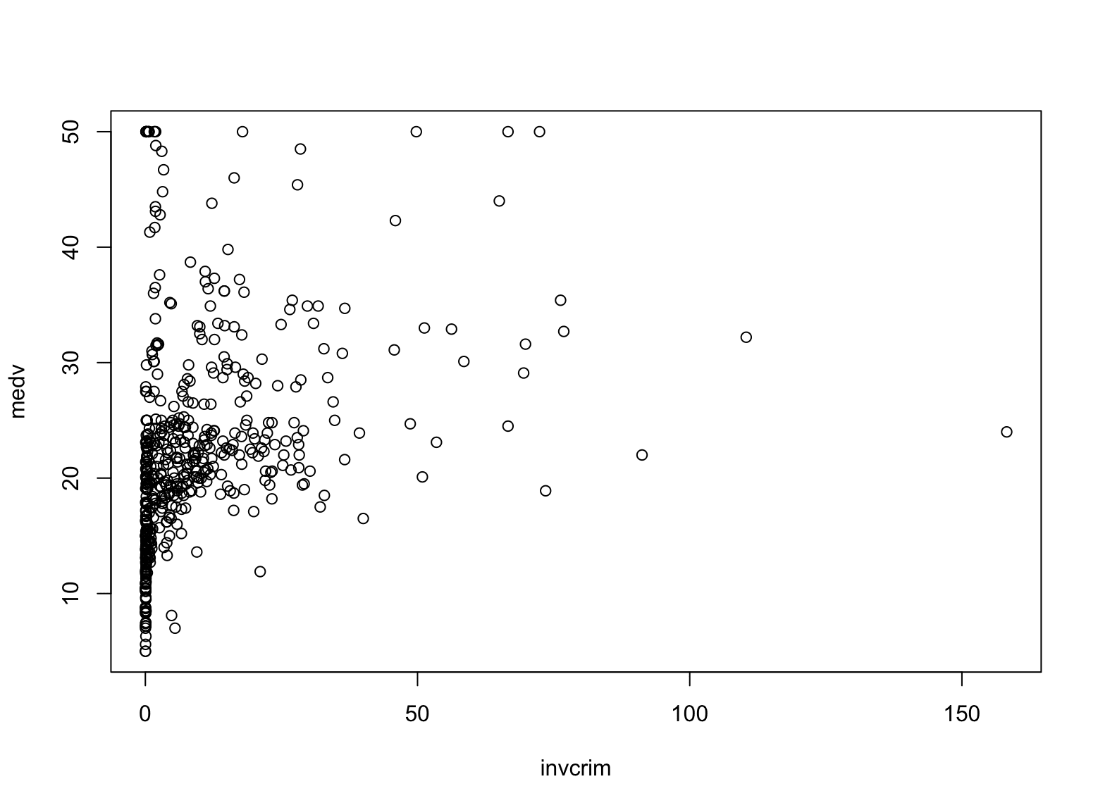
This doesn’t look like to have a trend. So you may also want to see if a segment of the data can show a trend. Let’s say, if you take only the subset of age column greater than 50. That’s what the filter() function can help:
|
1 |
Boston |> filter(age > 50) |> select(c(crim, medv)) |> plot() |
These are handy tools provided by dplyr. In this particular dataset, the trend is not trivial to discover in this ad-hoc way. You should look for more advanced techniques but these are the good starting point.
Besides exploring data visually, you can also explore the data numerically. The easiest way of dealing with data frame is to use the summary() function:
|
1 |
summary(Boston) |
This works for all numerical columns. You should see the basic statistics of each columns, including the maximum, minimum, median, mean, and so on. However, sometimes you want to see how different columns are correlated. For example, the chas column in this dataset indicates whether the location is near Charles River. It has a value of either 0 or 1. You can tell how the home value is related to such indicator variable using group_by():
|
1 |
group_by(boston, chas) |> summarize(avg=mean(medv), sd=sd(medv)) |
The group_by() function elevates a data frame into groups, which each group is a subset of rows with the same value in the chas column. Then the summarize() function creates a new column with a value computed from each group.
The output of the above is as follows:
|
1 2 3 4 5 |
# A tibble: 2 × 3 chas avg sd <int> <dbl> <dbl> 1 0 22.1 8.83 2 1 28.4 11.8 |
In fact, the summarize() function can be used without group_by(), but that will apply to the entire data frame; hence the output will only be one row.
Further Readings
This section provides you some links to study further on the materials above:
Online materials
- Data transformation with dplyr cheatsheet
- Introduction to dplyr from tidyverse
- The Boston Housing Dataset
Books:
- Beginning data science in R 4, second edition by Thomas Mailund
Summary
The library dplyr is a powerful package for data manipulation. In this post, you saw how you can use it to filter, select, and summarize data, and how the tools can help you explore a dataset. In particular, you learned:
- Using tibble as a different way of presenting abbrev
Photo by Airam Dato-on. Some rights reserved.
iated data frame
- How to manipulate tabular data by rows and columns
- How to perform group-by operations and compute aggregated values in a data frame


")
No comments yet.