
In this article, you will learn how to benchmark a deterministic 3-Tiered Graph-RAG system against a standard vector RAG pipeline on fact-dense queries, and what the results reveal about matching prompt complexity to model capacity.
Topics we will cover include:
- How to build a synthetic, fact-dense sports dataset that intentionally introduces noisy, contradictory text into a vector database while keeping ground truth in a graph store.
- How to implement and compare two retrieval functions — one for standard vector RAG and one for the 3-Tiered Graph-RAG — using ChromaDB and a local Flan-T5 model.
- Why a small-capacity local LLM can underperform with complex, conflict-resolution prompts, and what this means for production RAG system design.
Introduction
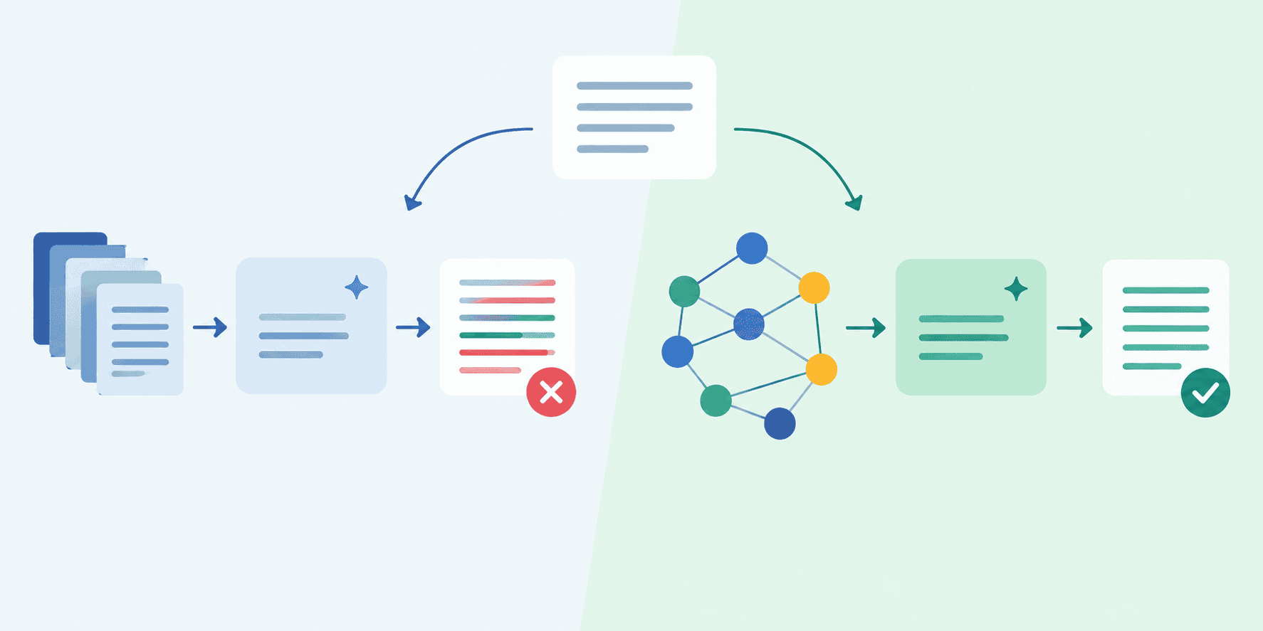
In a previous article, a deterministic, 3-Tiered Graph-RAG system architecture was proposed to address “lossiness” in dense vector databases when dealing with atomic facts. Because semantic proximity vector search and retrieval rely on similarity, classical RAG pipelines often confuse numeric data, historical stats, or entity relationships when several similar entities coexist in a latent space.
The proposed architecture tackled this limitation through a layered approach consisting of:
- A lightweight QuadStore knowledge graph based on a SPOC (Subject-Predicate-Object-Context) schema.
- A standard ChromaDB vector database capable of managing fuzzy, long-tail contexts.
In production-oriented engineering, however, hard numbers are critical. Accordingly, we now illustrate a benchmark between standard Vector RAG and our 3-Tiered Graph-RAG to measure how much reduction in hallucinations can be expected when querying over a fact-dense dataset.
Prerequisites and Setup
To run the example benchmark in this article, you’ll need to install these libraries if you don’t have them in your IDE — if you try the example out in a Google Colab notebook, install them all, as follows:
|
1 |
!pip install -q chromadb transformers |
Next, we import all the modules and functions we will need and set up a local LLM, in particular, the google/flan-t5-base model available with Hugging Face’s transformers library:
|
1 2 3 4 5 6 7 8 9 10 11 12 13 |
import chromadb from transformers import AutoModelForSeq2SeqLM, AutoTokenizer import random print("Initializing local, free-tier LLM (flan-t5-base)...") tokenizer = AutoTokenizer.from_pretrained("google/flan-t5-base") model = AutoModelForSeq2SeqLM.from_pretrained("google/flan-t5-base") def llm(prompt): """Wrapper to generate text directly from the local model""" inputs = tokenizer(prompt, return_tensors="pt") outputs = model.generate(**inputs, max_new_tokens=15) return tokenizer.decode(outputs[0], skip_special_tokens=True) |
Next, we build a simple QuadStore, following the same principles and guidelines as the one shown in the previous article:
|
1 2 3 4 5 6 7 8 9 10 11 |
class SimpleQuadStore: def __init__(self): self.facts = set() def add(self, subject, predicate, obj, context): self.facts.add((subject, predicate, str(obj), context)) def query(self, subject): return [f for f in self.facts if f[0] == subject] qs = SimpleQuadStore() |
Likewise, we need to initialize a Vector DB. We do this by instantiating a local ChromaDB collection that will handle unstructured chunks of text.
|
1 2 |
chroma_client = chromadb.Client() collection = chroma_client.create_collection(name="sports_stats") |
Next, we get some fresh data — and for this example, it couldn’t be fresher: we synthetically create it from scratch. The following code generates a synthetic dataset with performance information for 50 basketball players. It is designed to inject accurate truths into the graph database while intentionally feeding messy, contradictory paragraphs into the vector DB, just as often happens in the real-world texts that RAG systems are built upon.
|
1 2 3 4 5 6 7 8 9 10 11 12 13 14 15 16 17 18 19 20 21 22 23 24 25 |
benchmark_queries = [] print("Populating databases with synthetic sports data...") for i in range(50): player = f"Player_{i}" real_ppg = str(random.randint(15, 30)) fake_half = str(random.randint(2, 10)) fake_career = str(random.randint(11, 14)) # Graph DB receives the absolute truth qs.add(player, "season_ppg", real_ppg, "Sports_DB") # Vector DB receives messy unstructured text with multiple numbers text = ( f"During the recent game, {player} had a terrible first half, scoring only {fake_half} points. " f"Historically, his career average sat around {fake_career}. " f"However, his official season average PPG is currently {real_ppg}." ) collection.add(documents=[text], ids=[f"doc_{i}"]) benchmark_queries.append({ "question": f"What is the official season average PPG for {player}?", "entity": player, "true_answer": real_ppg }) |
We are almost there. Before running the benchmarking pipeline, the two missing pieces are the retrieval functions — one for each system. The standard RAG uses a simple context prompt, while the 3-Tiered Graph-RAG employs a strict rule-based prompt that forces the LLM to give first priority to graph facts over vector fallbacks.
|
1 2 3 4 5 6 7 8 9 10 11 12 13 14 15 16 17 |
def standard_vector_rag(q): # Simulating real-world context pollution by pulling top 3 similar chunks results = collection.query(query_texts=[q], n_results=3) context = " ".join(results["documents"][0]) # Joining the 3 paragraphs together prompt = f"Context: {context}\nQuestion: {q}\nAnswer strictly with the exact number:" return llm(prompt) def deterministic_3_tier_rag(q, entity): graph_res = qs.query(entity) p1_context = f"{entity} season average PPG is {graph_res[0][2]}" if graph_res else "None" p3_context = collection.query(query_texts=[q], n_results=1)["documents"][0][0] prompt = f"""Context 1 (Absolute Truth): {p1_context} Context 2 (Fallback Text): {p3_context} Question: {q} Answer strictly using Context 1 with the exact number:""" return llm(prompt) |
To run the benchmark, we loop through all 50 test queries in the dataset, check whether the text produced by the model contains the exact target number, and calculate overall accuracy.
|
1 2 3 4 5 6 7 8 9 10 11 12 |
print("\n--- RUNNING EVALUATION ---") v_correct, g_correct = 0, 0 for item in benchmark_queries: # We check if the true numeric string is anywhere in the LM's output if item["true_answer"] in standard_vector_rag(item["question"]): v_correct += 1 if item["true_answer"] in deterministic_3_tier_rag(item["question"], item["entity"]): g_correct += 1 print(f"Standard Vector-RAG Accuracy: {(v_correct / 50) * 100:.1f}%") print(f"3-Tiered Graph-RAG Accuracy: {(g_correct / 50) * 100:.1f}%") |
Final results:
|
1 2 3 |
--- RUNNING EVALUATION --- Standard Vector-RAG Accuracy: 96.0% 3-Tiered Graph-RAG Accuracy: 92.0% |
Summary of Results and Conclusion
These results carry a crucial lesson for production engineering of RAG systems: prompt complexity and model capacity must be matched. The google/flan-t5-base model is well-optimized but relatively small (250M parameters). In practice, this means it excels at straightforward reading comprehension in a standard RAG pipeline, but struggles with the complex instruction following required to handle conflicting data sources — exactly the kind found in the Graph-RAG prompt. The slight accuracy drop shows that enforcing graph-based rules via prompting requires a much larger reasoning model, such as Llama 3 or GPT-4. Forcing complex conflict-resolution prompts onto lighter, local LLMs can hurt performance in unexpected ways. These are not the results you might expect, but they shed light on the real-world trade-offs between different RAG approaches.




No comments yet.