In this article, you will learn how sentence embeddings work and how to build a fully client-side semantic search engine using Transformers.js, with no server, no API key, and no backend infrastructure required.
Topics we will cover include:
How sentence embeddings and cosine similarity form the foundation of semantic search.
How to generate and cache embeddings using the Transformers.js feature-extraction pipeline, including batching and Web Worker offloading.
How to build a complete, reusable SemanticSearch class and persist its index across page loads.
Building Semantic Search with Transformers.js and Sentence Embeddings
Introduction
You’ve probably shipped this bug before, where a user types “affordable laptop” into your search bar and gets zero results. But you know the database has dozens of laptop articles. They’re just all titled “budget notebook.” The words are different. The meaning is identical. Keyword search treats both as unrelated strings.
This isn’t an edge case. It’s the core limitation of keyword matching: it compares characters, not concepts. It doesn’t know that “cancel” and “return” describe related actions, that “broken” and “defective” mean the same thing, or that “I can’t log in” and “account access issue” are the same problem phrased two different ways.
What Sentence Embeddings Actually Are
Semantic search fixes this by comparing meaning. And with Transformers.js, you can build it entirely in the browser with no server, no API key, and no backend infrastructure. This tutorial walks through the full pipeline: how sentence embeddings work, how to generate them, how cosine similarity scores relevance, and how to wire it all into a working knowledge base search application.
A transformer model cannot process raw text. Before any computation happens, a sentence needs to become numbers. Embeddings are the result of that conversion: a sentence represented as a list of floating-point values called a vector.
The key property isn’t just that sentences become numbers. It’s that sentences with similar meaning become vectors that are geometrically close to each other in the same vector space.
The model used throughout this tutorial, sentence-transformers/all-MiniLM-L6-v2, maps every sentence to a point in a 384-dimensional vector space. The model was fine-tuned on over 1 billion sentence pairs specifically to learn this geometric property. “I need to cancel my order” and “How do I return a product?” end up close together. “The weather is beautiful today” ends up far from both.
The 384 dimensions aren’t human-readable. You can’t look at dimension 47 and say what it encodes. What matters for search is not any individual dimension but the distance between two vectors. Short distance means similar meaning. Large distance means unrelated.
A 3D scatter plot diagram illustrating how semantically similar sentences cluster together in vector space (click to enlarge)
Pooling and Normalization
The raw transformer model outputs one vector per token; every word and subword in a sentence gets its own vector. For semantic search, you need one vector per sentence.
Mean pooling handles this by averaging all token vectors, weighted by the attention mask, so padding tokens don’t contribute. Normalization then scales the result to unit length (magnitude = 1), which simplifies the similarity calculation covered in the next section.
In Transformers.js, both happen automatically when you pass { pooling: ‘mean’, normalize: true } to the pipeline call. Without these options, you get token-level embeddings, which are useful for tasks like named entity recognition, but not for sentence-level search.
The Feature-Extraction Pipeline
The feature-extraction task is different from every other Transformers.js pipeline. Tasks like text-classification or question-answering return human-readable outputs: labels, scores, strings. feature-extraction returns the raw vector representations that the model computed internally. You’re working one level lower, getting the numbers that all higher-level tasks are built on top of.
pipeline() downloads and initializes the model on first run (the browser caches it after that, so subsequent page loads are instant)
You then call the extractor with a string and the two options that give you a single, normalized sentence vector
The result is a Tensor object; calling .tolist()[0] converts it to a plain JavaScript array of 384 numbers you can work with directly
Understanding the Output Tensor
The Tensor object returned by feature-extraction has three fields worth knowing:
dims is the shape [n_sentences, 384]. Pass one sentence and dims[0] is 1. Pass ten sentences in a batch and dims[0] is 10. The second dimension is always 384 for this model
type is ‘float32‘, meaning each of the 384 values is a 32-bit floating-point number
data is a Float32Array containing all the numbers in row-major order. For a batch of 3 sentences, this is a flat array of 3 × 384 = 1,152 numbers
.tolist() converts the tensor to a nested JavaScript array, one inner array per sentence. output.tolist()[0] gives the vector for the first sentence as a plain array of 384 numbers.
Batching: Embed Multiple Sentences at Once
Passing an array of strings to the extractor processes all of them in a single model call. This is significantly faster than calling the pipeline once per sentence, because the transformer processes all inputs in parallel within one forward pass.
1
2
3
4
5
6
7
8
9
10
11
12
13
14
15
16
17
18
19
20
// Embed multiple documents in one call -- always prefer this over looping
constsentences=[
'How do I track my shipment?',
'What is your return policy?',
'How can I reset my password?',
'Do you offer international delivery?'
];
constbatchOutput=await extractor(sentences,{
pooling:'mean',
normalize:true
});
// batchOutput.dims = [4, 384] -- 4 sentences, each with 384 dimensions
console.log(`Batch shape:[${batchOutput.dims}]`);
// Convert to array of arrays -- one 384-element array per sentence
constvectors=batchOutput.tolist();
console.log(`Number of vectors:${vectors.length}`);// 4
Instead of four separate extractor() calls, one call handles all four sentences simultaneously
The transformer architecture is optimized for batched input, so the time it takes to embed 10 sentences together is much closer to embedding 1 sentence than to embedding 10 individually
Batching is the most important performance decision in a semantic search system. When indexing a corpus of 50 documents, one batch call is far faster than 50 individual calls. The difference compounds as your corpus grows.
Cosine Similarity: The Math Behind the Search
Once you have vectors for your documents and a vector for the search query, you need a way to measure how similar any two vectors are. That’s what cosine similarity does.
Cosine similarity measures the angle between two vectors. A score of 1.0 means the vectors point in the same direction (identical meaning). A score of 0 means they’re completely unrelated. Because we used normalize: true when generating embeddings, both vectors already have unit length (magnitude = 1), which simplifies the formula considerably:
1
2
3
4
cosine_similarity(A,B)=(A·B)/(|A|×|B|)
Since normalize:truesets|A|=|B|=1,thisbecomes:
cosine_similarity(A,B)=A·B=Σ(A[i]×B[i])
Just sum the element-wise products of the two vectors. That number is the cosine similarity. For sentence embeddings with mean pooling and normalization, practical scores fall roughly in these ranges:
Score Range
Interpretation
0.90 to 1.00
Near-identical meaning
0.70 to 0.90
Strong semantic match
0.50 to 0.70
Related topic, different angle
0.30 to 0.50
Loose connection
Below 0.30
Likely unrelated
Here’s the implementation:
1
2
3
4
5
6
7
8
9
10
11
12
13
14
15
16
17
18
19
20
21
22
23
24
25
26
27
28
29
30
/**
* Compute cosine similarity between two normalized vectors.
*
* This is just the dot product because normalize: true ensures
* both vectors already have unit length, making the denominator 1.
*
* @param {number[]|Float32Array} vecA - First normalized embedding vector
* @param {number[]|Float32Array} vecB - Second normalized embedding vector
* @returns {number} Similarity score between -1 and 1 (typically 0 to 1 for sentences)
dotProduct+=vecA[i]*vecB[i];// Multiply corresponding elements, then sum
}
// Clamp to [-1, 1] to handle floating-point rounding edge cases
returnMath.max(-1,Math.min(1,dotProduct));
}
// Example usage (assuming you've already run these through the extractor):
// cosineSimilarity(vecA, vecB) -- "I need to return a product" vs "How do I send an item back for a refund?"
// Result: ~0.82 (semantically similar)
//
// cosineSimilarity(vecA, vecC) -- "I need to return a product" vs "The stock market had a volatile week"
// Result: ~0.08 (unrelated)
What this code does:
The function loops through both 384-element vectors in parallel, multiplies corresponding values, and sums the results
That sum is the dot product, which equals cosine similarity when both vectors are normalized
The Math.max(-1, Math.min(1, …)) at the end handles the rare case where floating-point arithmetic produces a value like 1.0000002 due to rounding
Building a Semantic Search Class
The pattern for semantic search is always the same regardless of scale: embed documents once at startup, embed each query at search time, score every document against the query, sort by score.
The expensive step is generating the 384-number vector for each sentence. Caching those vectors in memory means subsequent searches only need to embed the query, which takes milliseconds.
1
2
3
4
5
6
7
8
9
10
11
12
13
14
15
16
17
18
19
20
21
22
23
24
25
26
27
28
29
30
31
32
33
34
35
36
37
38
39
40
41
42
43
44
45
46
47
48
49
50
51
52
53
54
55
56
57
58
59
60
61
62
63
64
65
66
67
68
69
70
71
72
73
74
75
76
77
78
79
80
81
82
83
84
85
86
87
88
89
90
91
92
93
94
95
96
97
98
99
100
101
102
103
104
105
106
107
108
109
110
111
112
113
/**
* SemanticSearch -- a simple client-side semantic search engine.
// Embed the search query -- the only model inference call during a search
constqueryOutput=await this.extractor(query,{
pooling:'mean',
normalize:true
});
constqueryVector=queryOutput.tolist()[0];
console.timeEnd('query embedding');
console.time('scoring');
// Score every indexed document against the query vector
// This is pure JavaScript math -- no model involved, so it's instant
constscored=this.index.map(doc=>({
doc,
score:cosineSimilarity(queryVector,doc.vector)
}));
// Sort descending -- highest relevance score first
scored.sort((a,b)=>b.score-a.score);
console.timeEnd('scoring');
// Return the top-k results, stripping the vector from the output
returnscored.slice(0,topK).map(({doc,score})=>({
id:doc.id,
title:doc.title,
text:doc.text,
metadata:doc.metadata,
score:score
}));
}
/**
* Serialize the index to JSON for storage in localStorage or IndexedDB.
* Saves the embedding step on subsequent page loads.
*/
toJSON(){
returnJSON.stringify(this.index);
}
/**
* Restore a previously serialized index without re-embedding anything.
* Vectors are plain arrays in JSON and deserialize directly.
*/
fromJSON(json){
this.index=JSON.parse(json);
returnthis;
}
}
What this code does:
indexDocuments takes your array of document objects (each needs at minimum a text field), embeds all the text in one batch call, and stores the result in this.index
The spread operator (…doc) preserves any metadata you pass in, so nothing gets dropped
search embeds only the query (one inference call, typically under 100ms), then runs cosineSimilarity against every cached document vector in a plain JavaScript loop. There’s no further model inference during scoring, which is why search feels instant after indexing completes
The toJSON and fromJSON methods let you persist the index across page loads, skipping the embedding step entirely on return visits
Full Working Demo: Knowledge Base Search
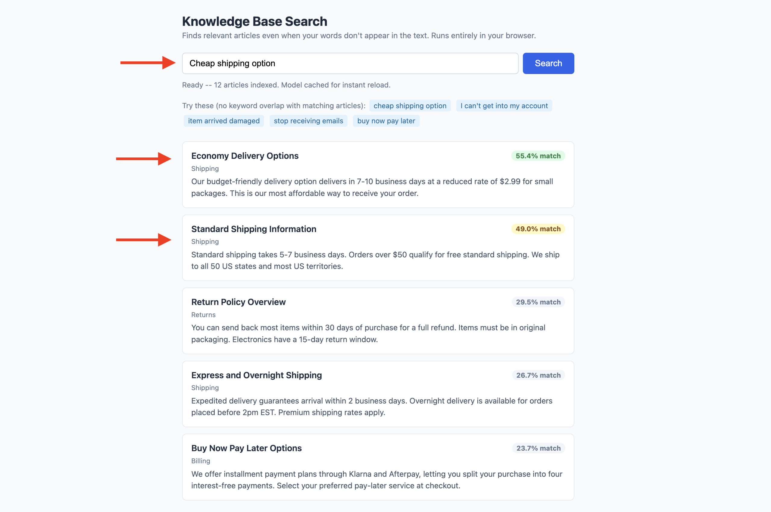
The application below is complete and self-contained. Copy it into a .html file, open it in any modern browser, and it works. The application uses 12 FAQ entries from a fictional e-commerce support knowledge base. The example queries are intentionally written with zero keyword overlap with the matching documents to demonstrate that semantic search is doing real work.
When the page loads, init() runs immediately. It creates the feature-extraction pipeline with a progress callback that updates the status line during the model download. Once the model is ready, indexDocuments embeds all 12 articles in one batch call and stores the vectors in memory. The search input and button are disabled until that step finishes, so users can’t trigger a search mid-index
When the user searches, search() embeds only the query (one inference call, typically under 100ms), then loops through all 12 cached document vectors, computing cosine similarity for each. That scoring loop is pure JavaScript arithmetic with no model involved, so it finishes in under a millisecond. Results are rendered sorted by score with color-coded match percentage badges
The example queries demonstrate the key capability. “Cheap shipping option” returns “Economy Delivery Options” at the top despite sharing zero keywords.
Running Inference in a Web Worker
The demo above runs all model inference on the main browser thread. For internal tools and demos, this is fine. For a user-facing production app, it’s not: model loading and embedding generation block the main thread, meaning scroll, input, and animations all freeze while inference is running. On older hardware, the browser may display an “unresponsive page” warning.
Web Workers solve this by running JavaScript in a background thread. The main thread stays responsive while the Worker handles all model work.
The Worker file (embedder-worker.js):
1
2
3
4
5
6
7
8
9
10
11
12
13
14
15
16
17
18
19
20
21
22
23
24
25
26
27
28
29
30
31
32
33
34
35
36
37
38
39
40
41
42
43
44
45
46
47
48
49
50
51
52
53
// embedder-worker.js
// Runs in a background thread -- has no access to the DOM.
The Worker uses a singleton pattern (getExtractor() creates the pipeline once and returns it on subsequent calls) to avoid re-downloading the model if multiple messages arrive in quick succession
The id field on each message is a correlation key: when the Worker sends back an embed_result, the main thread uses the id to find the matching Promise in the pending Map and resolve it. Without this, if two embedding requests were in flight at the same time, you couldn’t tell which result belonged to which request
The pending Map stays small (one entry per in-flight request) and cleans up after itself as responses arrive
Persisting the Index Across Page Loads
Computing embeddings is the slow step. For a document corpus that doesn’t change between visits, you can serialize the index to JSON and store it in localStorage, so the next page load skips the embedding step entirely.
1
2
3
4
5
6
7
8
9
10
11
12
13
14
15
16
17
// After indexing -- save to localStorage
constserialized=JSON.stringify(searcher.index);
localStorage.setItem('kb-index',serialized);
localStorage.setItem('kb-index-version','2025-06-01');// Update this when content changes
// On page load -- restore the index if it exists and is still current
// Vectors are plain arrays in JSON -- no special deserialization needed
console.log('Index restored from cache, skipping embedding step');
}
}
localStorage handles around 5 MB, depending on the browser. For 12 documents with 384-dimensional float vectors, the serialized index is roughly 200 KB, well within the limit. For larger corpora, IndexedDB has no practical size constraint and works the same way with a slightly more verbose API.
Scaling Beyond a Few Hundred Documents
The approach above scores every document per query. That works well up to a few hundred documents before latency starts to show. For larger corpora, the official Transformers.js examples repository includes a pglite-semantic-search demo that runs an in-browser PostgreSQL instance with the pgvector extension for approximate nearest neighbor search, which is meaningfully faster than brute-force scoring for large collections while still keeping everything client-side.
Choosing the Right Model
Xenova/all-MiniLM-L6-v2 is the right default for most English-language use cases. It’s fast, small, and produces strong results for semantic search. The table below covers the main options:
For multilingual use cases where a knowledge base has content in French, German, and English simultaneously, multilingual-e5-small handles cross-lingual queries. A user searching in English will surface relevant documents written in French because the model maps equivalent meanings to nearby vectors regardless of language.
Conclusion
The pipeline is four steps: load the model once, embed your document corpus in a batch, embed each query at search time, score with cosine similarity, and sort. Everything in this tutorial runs from a single CDN import with no server, no API key, and no data leaving the user’s device.
The same core concepts — vectors, similarity, and ranking — are also the foundation of recommendation systems, duplicate content detection, clustering, and retrieval-augmented generation. Each of those applications is built on the same feature-extraction pipeline and cosineSimilarity function covered here. Start with the knowledge base demo, extend the corpus to your own documents, and those more advanced patterns will make sense quickly once you’ve seen the basics working.


No comments yet.