Train Your Large Model on Multiple GPUs with Tensor Parallelism

Tensor parallelism is a model-parallelism technique that shards a tensor along a specific dimension. It distributes the computation of a tensor across multiple devices with minimal communication overhead. This technique is suitable for models with very large parameter tensors where even a single matrix multiplication is too large to fit on a single GPU. In this article, you will learn how to use tensor parallelism. In particular, you will learn about:

• What is tensor parallelism
• How to design a tensor parallel plan
• How to apply tensor parallelism in PyTorch

Let’s get started!

Train Your Large Model on Multiple GPUs with Tensor Parallelism.
Photo by Seth kane. Some rights reserved.

Overview

This article is divided into five parts; they are:

• An Example of Tensor Parallelism
• Setting Up Tensor Parallelism
• Preparing Model for Tensor Parallelism
• Train a Model with Tensor Parallelism
• Combining Tensor Parallelism with FSDP

An Example of Tensor Parallelism

Tensor parallelism originated from the Megatron-LM paper. This technique does not apply to all operations; however, some, such as matrix multiplication, are implemented using sharded computation.

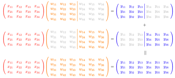
Column-wise tensor parallel: You sharded the weight $\mathbf{W}$ into columns, and applied the matrix multiplication $\mathbf{XW}=\mathbf{Y}$ to produce sharded output that needs to be concatenated.

Let’s consider a simple matrix-matrix multiplication operation as follows:

It is a $3\times 4$ matrix $\mathbf{X}$ multiplied by a $4\times 6$ matrix $\mathbf{W}$ to produce a $3\times 6$ matrix $\mathbf{Y}$. You can indeed break it down into two matrix multiplications, one is $\mathbf{X}$ times a $4\times 3$ matrix $\mathbf{W}_1$ to produce a $3\times 3$ matrix $\mathbf{Y}_1$, and the other is $\mathbf{X}$ times another $3\times 2$ matrix $\mathbf{W}_2$ to produce a $3\times 3$ matrix $\mathbf{Y}_2$. Then the final $\mathbf{Y}$ is the concatenation of $\mathbf{Y}_1$ and $\mathbf{Y}_2$.

You can see that in this case, you do not need to host the large matrix $\mathbf{W}$ but work on a smaller split of it. This saves memory. The output of each split is smaller, hence it also communicates faster to other devices.

The case above is called column-wise parallel. You can generalize this to have more than two splits of the matrix $\mathbf{W}$ along the column dimension.

Another variation is row-wise parallel, which is illustrated as follows:

Row-wise tensor parallel: You sharded the weight $\mathbf{W}$ into rows, and applied the matrix multiplication $\mathbf{XW}=\mathbf{Y}$ to produce partial outputs that need to be added elementwise.

With the same $\mathbf{XW}=\mathbf{Y}$ matrix multiplication, you now split $\mathbf{X}$ into columns and split $\mathbf{W}$ into rows. In the illustration above, a $3\times 2$ matrix from the left half of $\mathbf{X}$ multiplies by a $2\times 6$ matrix from the upper half of $\mathbf{W}$ to produce a $3\times 6$ matrix. The output shape is the same as the full equation, but the values only correspond to the upper half of $\mathbf{W}$. Repeating the same operation with the right half of $\mathbf{X}$ and the lower half of $\mathbf{W}$, then summing the two results, gives you the final output $\mathbf{Y}$.

In row-wise parallel, you work with splits of both $\mathbf{X}$ and $\mathbf{W}$. The workload is lighter than performing the full matrix multiplication. The output is larger than with column-wise parallel, requiring more bandwidth to communicate the result to other devices.

Not all operations in your deep learning model are matrix multiplications. Therefore, tensor parallelism does not work on every element in your model. Some operations, such as activation functions or normalization layers, can be parallelized differently. For operations that cannot be parallelized, your model must compute them in their original form.

Tensor parallelism offers benefits beyond memory savings—it provides fine-grained control over computation and communication patterns. Since matrix multiplications are sharded, you can control whether to unshard the result, allowing you to avoid communication overhead when working directly with sharded DTensor objects.

Setting Up Tensor Parallelism

Tensor parallelism in PyTorch is a part of the distributed framework. Therefore, the script is launched with the torchrun command as in the case of distributed data parallelism, pipeline parallelism, and fully sharded data parallelism. You need to initialize the distributed environment as usual, but you also need to set up the device mesh:

The device mesh is a high-level abstraction of the process group. You will see why it is needed in later sections. It is necessary because you use the mesh to wrap a model into a tensor parallel model, using the following syntax:

Afterward, some of the model’s weights will be replaced with DTensor objects, enabling parallel execution. Distributed collective operations such as all-gather, all-reduce, and reduce-scatter may be performed internally to make the model work as if it were on a single device. These details are transparent to you.

Preparing Model for Tensor Parallelism

Let’s see how to run the training script from the previous article with tensor parallelism.

Converting a model to run with tensor parallelism does not require changing the model architecture. Instead, you need to know the fully-qualified name of each module and submodule in your model. These are the same as the keys in your model’s state_dict(), or you can revisit your model architecture code to find the module names.

You need to identify those names to create a parallelization plan. It is a Python dictionary that maps module names to ParallelStyle objects. Below is an example:

The model architecture code is identical to that in the previous article. The dictionary tp_plan is created from the perspective of a transformer block. Note that each block is declared as:

From the perspective of the class LlamaDecoderLayer, you can find an nn.Linear layer as layer.mlp.gate_proj, hence you use the key mlp.gate_proj in the tp_plan dictionary to reference it.

When you use tensor parallelism, you should be aware that PyTorch does not know how to parallelize an arbitrary module, such as the custom module that you defined. But a few standard modules have concrete implementations of tensor parallelism:

• nn.Linear and nn.Embedding: You can use ColwiseParallel and RowwiseParallel to parallelize them. The operation is described above.
• nn.LayerNorm, nn.RMSNorm, and nn.Dropout: You can use SequenceParallel to parallelize them.

As PyTorch is evolving, refer to the official documentation for the latest coverage of tensor parallelism.

Once you set up tp_plan, you can apply it to the model using the parallelize_module() function. This replaces the module’s parameters with DTensor objects and makes the module run sharded computations as if it were on a single device. The for-loop above applies parallelize_module() to each transformer block for convenience. You can also apply it to the full base model, but you would need to update tp_plan with considerable repetition, since transformer blocks are repeated many times in the base model.

The transformer block contains two RMS norm layers. You mark them with SequenceParallel to indicate they should be sharded on the sequence dimension (dimension 1 of the input tensor).

The transformer block contains several nn.Linear layers: three in the feed-forward sublayer and four in the attention sublayer. You can mark them with either ColwiseParallel or RowwiseParallel to parallelize them, but there are some considerations:

• ColwiseParallel by default expects a full tensor as input, and the output is sharded on the last dimension, making the output tensor smaller.
• RowwiseParallel by default expects a tensor sharded on the last dimension as input, and the output is a full-sized tensor, the same size as if it were not parallelized.

This is why you specify:

In the feed-forward sublayer, you project the input tensor to $4\times$ larger in the last dimension (using gate_proj and up_proj) and apply SwiGLU activation, then project the result back to the original size (using down_proj). Using ColwiseParallel for gate_proj and up_proj reduces the output tensor size and reduces communication overhead. You do not need to send the output to another device since the next layer, down_proj, uses RowwiseParallel and expects a tensor sharded on the last dimension as input—the output from ColwiseParallel fits perfectly. This demonstrates how to design a tensor parallel plan for your model.

The output from a RowwiseParallel layer defaults to a full-sized DTensor object, but you can change this requirement in the tp_plan for the down_proj layer to make it sharded on dimension 1. The tensor parallelism engine will determine the required communication operations. The reason for sharding on dimension 1 is that the next layer in the larger model is the RMS norm layer from the subsequent transformer block, and you need to prepare the tensor for that layer.

Adding input_layouts or output_layouts allows you to override the default behavior of ColwiseParallel and RowwiseParallel. This explains why you set the plan for the nn.Linear layers in the attention sublayer:

The Q/K/V projection outputs will be used with grouped-query attention (GQA). You use F.scaled_dot_product_attention() to compute the attention scores, but the way it is used in the LlamaAttention class, along with various tensor transpose and reshape operations, does not work well with distributed tensors. Therefore, you set the output to Replicate() to force a full copy to each device. Correspondingly, the input to o_proj will be a full tensor from the attention output, so you set input_layouts=Replicate(). Similarly, since the output from o_proj will be the input to the RMS norm, you set output_layouts=Shard(1) to make it compatible.

One more consideration: Since this is a pre-norm model, the inputs to the attention and feed-forward sublayers are outputs from the RMS norm, which are sharded on the sequence dimension. However, the first operation in both sublayers is a matrix multiplication with ColwiseParallel. You need to transform a tensor sharded on dimension 1 into a full tensor when passing it to the sublayers. This is why you use PrepareModuleInput to annotate the two sublayers:

The attention sublayer is defined as follows:

The forward() function of LlamaAttention takes three arguments. In LlamaDecoderLayer, you call the attention sublayer with hidden_states as a positional argument and rope and attn_mask as keyword arguments. If you were to use the LlamaAttention class with all keyword arguments, that is, self.self_attn(hidden_states=hidden_states, rope=rope, attn_mask=attn_mask), you would set input_kwarg_layouts and desired_input_kwarg_layouts instead of input_layouts and desired_input_layouts. Since your usage pattern has only one positional argument, you set input_layouts=Shard(dim=1) to indicate that you expect a DTensor sharded on dimension 1 as input.

There are also PrepareModuleOutput and PrepareModuleInputOutput if you need to override the DTensor layout in other cases.

Some other elements in the top-level model can be parallelized. So you can create a second plan and apply it to the top-level model:

By now, your model is parallelized. You can check that this is the case by verifying a special attribute on an element that is parallelized:

Train a Model with Tensor Parallelism

That’s all you need for tensor parallelism. You set up the data loader, optimizer, learning rate scheduler, and loss function as usual, and nothing else needs to change in the training loop. It works because the input tensor is replicated across the mesh, and the embedding layer shards the tensor initially. As the input propagates through the model, it reaches the prediction head lm_head, which produces a replicated tensor as output. The loss can then be computed as usual, and gradient updates are applied to the DTensor objects.

However, you can go one step further by having the model produce a sharded tensor as output, then compute the loss on that tensor. This only works for cross-entropy loss using F.cross_entropy() or nn.CrossEntropyLoss(), which is the case here. You need to update the tensor parallel plan:

Note that the output of the final layer, lm_head, uses ColwiseParallel with output_layouts set to the default, which is sharded along the last dimension. You also set use_local_output=False to keep the output as a DTensor object. In the training loop, you need to wrap the loss calculation as follows:

This way, you pass the reference tensor target_ids to each device in the tensor parallel device mesh, and each device computes its corresponding loss based on its shard of logits. The gradient is then computed from each shard in a parallelized backward pass. Once computed and stored as a sharded tensor, the optimizer updates the weights as usual.

The final piece of the training script involves saving and loading model checkpoints. Since you are running distributed training, use the distributed checkpointing API as mentioned in the previous article.

For completeness, below is the full script for running tensor parallelism training:

You should run this code with the torchrun command, such as:

Combining Tensor Parallelism with FSDP

Tensor parallelism is a form of model parallelism: the model runs separately on each device, with distinct operations. Data parallelism replicates the model across multiple devices, each performing the same operations on different data.

You can combine tensor parallelism with data parallelism to achieve 2D parallelism. It is straightforward to integrate with FSDP with only a few lines of code.

Before you begin, you must determine how tensor and data parallelism should interact. This is called 2D parallelism because you can consider your GPU cluster as a 2D grid:

$$
\begin{bmatrix}
\text{GPU}(0,0) & \text{GPU}(0,1) \\
\text{GPU}(1,0) & \text{GPU}(1,1) \\
\end{bmatrix}
$$

You now number each device as a pair of indices, such as $(0,1)$. The first index is usually the data-parallel index, and the second is the tensor-parallel index. If you have multiple GPUs across multiple nodes, the first index typically represents the node index, and the second represents the GPU index on that node. This is why it’s called a device mesh. You can define a mesh for 2D parallelism as follows:

With this mesh, you apply tensor parallelism only to the tensor-parallel dimension. You can do this by using a submesh with parallelize_module() as follows:

After converting the model to a tensor parallel model, you can further apply FSDP using the data parallel dimension submesh:

This is essentially an FSDP model, so you need to set up the data loader accordingly using a DistributedSampler:

Note that the DistributedSampler is repeated as many times as the data parallel size. Correspondingly, the batch_size is divided by the same number to maintain the same effective batch size.

The rest of the training script remains the same. Here’s how it works: When you pass a micro-batch of data to the model, it operates as an FSDP model, with each shard exchanging weights to create a temporary, unsharded model for processing. The FSDP model output is then combined to compute the loss.

Within the FSDP model, a tensor-parallel model is distributed across multiple devices. This device set is orthogonal to the FSDP dimension, and each FSDP shard forms a full tensor-parallel model. Each micro-batch is processed by the tensor-parallel model, in which each shard produces only a sharded output rather than a full output. You need to use all-gather to combine the sharded output or use loss parallelism to compute the loss on the sharded output.

In 2D parallelism, your model runs with two hierarchical levels of parallelism: first data parallelism, then tensor parallelism. The mesh design typically makes the first dimension (data parallel) inter-node and the second dimension (tensor parallel) intra-node to optimize performance. You can also replace FSDP with standard distributed data parallelism for a different 2D parallelism implementation. You can even create 3D parallelism by combining data, pipeline, and tensor parallelism in this hierarchical order, resulting in a 3D mesh grid.

For completeness, below is the full script for running 2D parallelism training using tensor parallelism and FSDP, and you still need to run it with torchrun: