Creating a Llama or GPT Model for Next-Token Prediction

By Adrian Tam on January 21, 2026 in Training Transformer Models 0

Natural language generation (NLG) is challenging because human language is complex and unpredictable. A naive approach of generating words randomly one by one would not be meaningful to humans. Modern decoder-only transformer models have proven effective for NLG tasks when trained on large amounts of text data. These models can be huge, but their structure is relatively simple. In this article, you will learn how to create a Llama or GPT model for next-token prediction.

Let’s get started.

Creating a Llama or GPT Model for Next-Token Prediction
Photo by Roman Kraft. Some rights reserved.

Overview

This article is divided into three parts; they are:

Understanding the Architecture of the Llama or GPT Model
Creating a Llama or GPT Model for Pretraining
Variations in the Architecture

Understanding the Architecture of the Llama or GPT Model

The architecture of a Llama or GPT model is simply a stack of transformer blocks. Each transformer block consists of a self-attention sub-layer and a feed-forward sub-layer, with normalization and residual connections applied around each sub-layer. That’s all the model has.

The architecture of GPT-2 and Llama models is shown in the figure below.

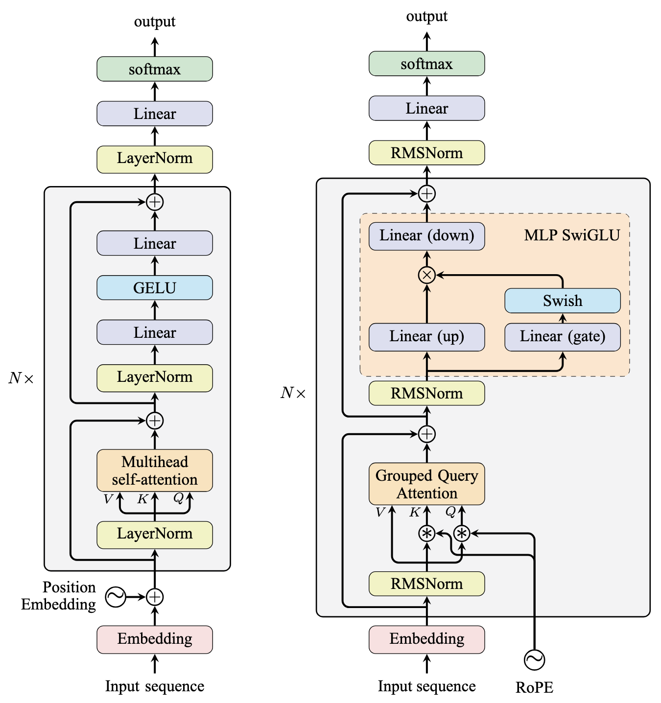
The GPT-2 (left) and Llama (right) model architectures

GPT-2 is older and mostly follows the architecture of the original encoder-decoder transformer. It uses layer normalization and multi-headed attention, along with two linear layers in the feed-forward sub-layer. GPT-2 differs from the original transformer design in:

Using pre-norm instead of post-norm
Using learned position embeddings instead of sinusoidal embeddings
Using GELU as the activation function in the feed-forward sub-layer instead of ReLU

Since GPT-2 is a decoder-only model, no encoder input is available, so the cross-attention sub-layer from the original transformer’s decoder stack is removed. However, you should not confuse its architecture with a transformer encoder because a causal mask is applied to the self-attention sublayer, forcing the model to attend only to the left context.

The Llama model revised several aspects of GPT-2, and versions 1 through 3 of Llama share the same architecture. Like GPT-2, the Llama model is a decoder-only model that uses pre-norm. However, unlike GPT-2, the Llama model:

Uses grouped query attention (GQA) instead of multi-headed attention (MHA)
Uses rotary position embeddings (RoPE) instead of learned position embeddings or sinusoidal position embeddings, and this is applied at each self-attention sub-layer.
Uses SwiGLU as the activation function in the feed-forward sub-layer instead of ReLU. As a result, the feed-forward sublayer has three linear layers and an element-wise multiplication.
Uses RMSNorm as the normalization function instead of LayerNorm

After the entire transformer stack, one more normalization layer is applied to the hidden state. The base model refers to the neural network from the input embedding through this final normalization layer.

For pretraining, you want the model to learn to predict the next token in a sequence. To do this, you add a pretraining head to the model—a linear layer that projects the hidden state to the vocabulary size. The softmax function is then used to get the probability distribution over the vocabulary.

Creating a Llama Model for Pretraining

There are many implementations of the Llama model available online. You can use existing code or create one using the Hugging Face transformers library if you care more about training results than understanding the model architecture. For example, the model created below is a Llama model with 12 layers and a pretraining head:

from transformers import LlamaForCausalLM, LlamaConfig

config = LlamaConfig(
    num_hidden_layers=12,
    hidden_size=768,
    num_attention_heads=12
)
model = LlamaForCausalLM(config=config)

from transformers import LlamaForCausalLM, LlamaConfig

config = LlamaConfig(

num_hidden_layers=12,

hidden_size=768,

num_attention_heads=12

)

model = LlamaForCausalLM(config=config)

However, creating a Llama model from scratch using PyTorch is not difficult. First, let’s define a data class to hold the model configuration:

import dataclasses

@dataclasses.dataclass
class LlamaConfig:
    vocab_size: int = 50000  # Size of the tokenizer vocabulary
    max_position_embeddings: int = 2048  # Maximum sequence length
    hidden_size: int = 768  # Dimension of hidden layers
    intermediate_size: int = 4*768  # Dimension of MLP's hidden layer
    num_hidden_layers: int = 12  # Number of transformer layers
    num_attention_heads: int = 12  # Number of attention heads
    num_key_value_heads: int = 3  # Number of key-value heads for GQA

import dataclasses

@dataclasses.dataclass

class LlamaConfig:

vocab_size: int = 50000 # Size of the tokenizer vocabulary

max_position_embeddings: int = 2048 # Maximum sequence length

hidden_size: int = 768 # Dimension of hidden layers

intermediate_size: int = 4*768 # Dimension of MLP's hidden layer

num_hidden_layers: int = 12 # Number of transformer layers

num_attention_heads: int = 12 # Number of attention heads

num_key_value_heads: int = 3 # Number of key-value heads for GQA

The model should have a fixed vocabulary size that matches the tokenizer you use. The maximum sequence length is a parameter for the rotary position embeddings and should be large enough to accommodate the longest sequence in your dataset. The hidden size, intermediate size, number of layers, and number of attention heads are hyperparameters that directly determine the model size and training or inference speed.

Rotary Position Embeddings

Let’s first implement the rotary position embeddings. Unlike other modules, rotary position embeddings have no learnable parameters. Instead, they precompute the cosine and sine matrices and save them as buffers. Right before attention is computed, RoPE is applied to the query and key matrices. In formula, RoPE is applied as:

$$
\begin{aligned}
Q_{s,i} &= Q_{s,i} \cos(s\theta_i) – Q_{s,\frac{d}{2}+i} \sin(s\theta_i) \\
Q_{s,\frac{d}{2}+i} &= Q_{s,i} \sin(s\theta_i) + Q_{s,\frac{d}{2}+i} \cos(s\theta_i)
\end{aligned}
$$

where $Q_{s,i}$ is the $i$-th element of the token embedding of the query matrix $Q$ at sequence position $s$. The length of the token embedding (also known as the hidden size or the model dimension) is $d$. Applying RoPE to the key matrix $K$ is similar. The frequency term $\theta_i$ is computed as:

$$
\theta_i = \frac{1}{10000^{2i/d}}
$$

To implement RoPE, you can use the following:

import torch.nn as nn

def rotate_half(x):
    """Rotates half the hidden dims of the input."""
    x1, x2 = x.chunk(2, dim=-1)
    return torch.cat((-x2, x1), dim=-1)

class RotaryPositionEncoding(nn.Module):
    def __init__(self, dim, max_position_embeddings):
        super().__init__()
        self.dim = dim
        self.max_position_embeddings = max_position_embeddings
        N = 10000.0
        inv_freq = 1.0 / (N ** (torch.arange(0, dim, 2) / dim))
        inv_freq = torch.cat((inv_freq, inv_freq), dim=-1)
        position = torch.arange(max_position_embeddings)
        sinusoid_inp = torch.outer(position, inv_freq)
        self.register_buffer("cos", sinusoid_inp.cos())
        self.register_buffer("sin", sinusoid_inp.sin())

    def forward(self, x):
        """Apply RoPE to tensor x"""
        batch_size, seq_len, num_heads, head_dim = x.shape
        dtype = x.dtype
        cos = self.cos.to(dtype)[:seq_len].view(1, seq_len, 1, -1)
        sin = self.sin.to(dtype)[:seq_len].view(1, seq_len, 1, -1)
        output = (x * cos) + (rotate_half(x) * sin)
        return output

import torch.nn as nn

def rotate_half(x):

"""Rotates half the hidden dims of the input."""

x1, x2 = x.chunk(2, dim=-1)

return torch.cat((-x2, x1), dim=-1)

class RotaryPositionEncoding(nn.Module):

def __init__(self, dim, max_position_embeddings):

super().__init__()

self.dim = dim

self.max_position_embeddings = max_position_embeddings

N = 10000.0

inv_freq = 1.0 / (N ** (torch.arange(0, dim, 2) / dim))

inv_freq = torch.cat((inv_freq, inv_freq), dim=-1)

position = torch.arange(max_position_embeddings)

sinusoid_inp = torch.outer(position, inv_freq)

self.register_buffer("cos", sinusoid_inp.cos())

self.register_buffer("sin", sinusoid_inp.sin())

def forward(self, x):

"""Apply RoPE to tensor x"""

batch_size, seq_len, num_heads, head_dim = x.shape

dtype = x.dtype

cos = self.cos.to(dtype)[:seq_len].view(1, seq_len, 1, -1)

sin = self.sin.to(dtype)[:seq_len].view(1, seq_len, 1, -1)

output = (x * cos) + (rotate_half(x) * sin)

return output

RoPE is a function to mutate the input tensor. To test the above RoPE module, you can do the following:

...
import torch

batch_size, seq_len, num_heads, head_dim = 1, 10, 4, 128
max_position_embeddings = 2048
x = torch.randn(batch_size, seq_len, num_heads, head_dim)
rope = RotaryPositionEncoding(head_dim, max_position_embeddings)
x_rope = rope(x)

...

import torch

batch_size, seq_len, num_heads, head_dim = 1, 10, 4, 128

max_position_embeddings = 2048

x = torch.randn(batch_size, seq_len, num_heads, head_dim)

rope = RotaryPositionEncoding(head_dim, max_position_embeddings)

x_rope = rope(x)

Self-Attention Sub-Layer

The self-attention sub-layer is the core of the transformer model. It is responsible for attending to the context of the input sequence. In the Llama model, grouped query attention (GQA) is used, in which the key and value matrices are projected to fewer heads than the query matrix.

You do not need to implement GQA from scratch, as PyTorch provides a built-in GQA implementation in the scaled_dot_product_attention function. You just need to pass the enable_gqa=True argument to the function.

Below is how you can implement the self-attention sub-layer:

lass LlamaAttention(nn.Module):
    def __init__(self, config):
        super().__init__()
        self.hidden_size = config.hidden_size
        self.num_heads = config.num_attention_heads
        self.head_dim = self.hidden_size // self.num_heads
        self.num_kv_heads = config.num_key_value_heads  # GQA: H_kv < H_q

        # hidden_size must be divisible by num_heads
        assert (self.head_dim * self.num_heads) == self.hidden_size

        # Linear layers for Q, K, V, and O projections
        self.q_proj = nn.Linear(self.hidden_size, self.num_heads * self.head_dim, bias=False)
        self.k_proj = nn.Linear(self.hidden_size, self.num_kv_heads * self.head_dim, bias=False)
        self.v_proj = nn.Linear(self.hidden_size, self.num_kv_heads * self.head_dim, bias=False)
        self.o_proj = nn.Linear(self.num_heads * self.head_dim, self.hidden_size, bias=False)

    def forward(self, hidden_states, rope, attn_mask):
        bs, seq_len, dim = hidden_states.size()

        # Project inputs to Q, K, V
        query_states = self.q_proj(hidden_states).view(bs, seq_len, self.num_heads, self.head_dim)
        key_states = self.k_proj(hidden_states).view(bs, seq_len, self.num_kv_heads, self.head_dim)
        value_states = self.v_proj(hidden_states).view(bs, seq_len, self.num_kv_heads, self.head_dim)

        # Apply rotary position embeddings
        query_states = rope(query_states)
        key_states = rope(key_states)

        # Transpose tensors from BSHD to BHSD dimension for scaled_dot_product_attention
        query_states = query_states.transpose(1, 2)
        key_states = key_states.transpose(1, 2)
        value_states = value_states.transpose(1, 2)

        # Use PyTorch's optimized attention implementation
        attn_output = F.scaled_dot_product_attention(
            query_states,
            key_states,
            value_states,
            attn_mask=attn_mask,
            dropout_p=0.0,
            enable_gqa=True,
        )

        # Transpose output tensor from BHSD to BSHD dimension, reshape to 3D, and then project output
        attn_output = attn_output.transpose(1, 2).reshape(bs, seq_len, self.hidden_size)
        attn_output = self.o_proj(attn_output)
        return attn_output

lass LlamaAttention(nn.Module):

def __init__(self, config):

super().__init__()

self.hidden_size = config.hidden_size

self.num_heads = config.num_attention_heads

self.head_dim = self.hidden_size // self.num_heads

self.num_kv_heads = config.num_key_value_heads # GQA: H_kv < H_q

# hidden_size must be divisible by num_heads

assert (self.head_dim * self.num_heads) == self.hidden_size

# Linear layers for Q, K, V, and O projections

self.q_proj = nn.Linear(self.hidden_size, self.num_heads * self.head_dim, bias=False)

self.k_proj = nn.Linear(self.hidden_size, self.num_kv_heads * self.head_dim, bias=False)

self.v_proj = nn.Linear(self.hidden_size, self.num_kv_heads * self.head_dim, bias=False)

self.o_proj = nn.Linear(self.num_heads * self.head_dim, self.hidden_size, bias=False)

def forward(self, hidden_states, rope, attn_mask):

bs, seq_len, dim = hidden_states.size()

# Project inputs to Q, K, V

query_states = self.q_proj(hidden_states).view(bs, seq_len, self.num_heads, self.head_dim)

key_states = self.k_proj(hidden_states).view(bs, seq_len, self.num_kv_heads, self.head_dim)

value_states = self.v_proj(hidden_states).view(bs, seq_len, self.num_kv_heads, self.head_dim)

# Apply rotary position embeddings

query_states = rope(query_states)

key_states = rope(key_states)

# Transpose tensors from BSHD to BHSD dimension for scaled_dot_product_attention

query_states = query_states.transpose(1, 2)

key_states = key_states.transpose(1, 2)

value_states = value_states.transpose(1, 2)

# Use PyTorch's optimized attention implementation

attn_output = F.scaled_dot_product_attention(

query_states,

key_states,

value_states,

attn_mask=attn_mask,

dropout_p=0.0,

enable_gqa=True,

)

# Transpose output tensor from BHSD to BSHD dimension, reshape to 3D, and then project output

attn_output = attn_output.transpose(1, 2).reshape(bs, seq_len, self.hidden_size)

attn_output = self.o_proj(attn_output)

return attn_output

This is a few lines of code, but not trivial. The attention block implements GQA self-attention with RoPE.

Upon entry, you project the input tensor to query, key, and value tensors using linear layers. Then split the last dimension (corresponding to the token embeddings) into two parts: one for the number of heads and one for the per-head dimension. Note that the original tensor has shape (batch_size, sequence_length, hidden_size), and after projection and reshaping, it has shape (batch_size, sequence_length, num_heads, head_dim). You should transpose this to (batch_size, num_heads, sequence_length, head_dim) before applying attention.

Computing GQA is straightforward. You simply call the scaled_dot_product_attention function with enable_gqa=True and pass the query, key, and value tensors. Note that the query tensor has more heads than the key and value tensors, but the number of query heads must be a multiple of the number of key and value heads.

For the output, you restore the tensor to its original shape and project it again with a linear layer.

SwiGLU Sub-Layer

The feed-forward sub-layer in the Llama model uses SwiGLU as the activation function. Mathematically, SwiGLU is defined as:

$$
\begin{aligned}
\text{SwiGLU}(x) &= \text{swish}(xW_1 + b_1) \otimes (xW_2 + b_2) \\
\text{swish}(x) &= \frac{x}{1 + e^{-x}}
\end{aligned}
$$

The symbol $\otimes$ represents element-wise multiplication of the two tensors. Effectively, the SwiGLU function models a quadratic function.

In GPT and Llama models, you expand the input tensor dimension to a larger size, apply the activation function, and then project it back to the original dimension. This dimensional expansion is believed to enable learning more complex relationships between input and output.

PyTorch does not provide a single function for implementing SwiGLU. But you can implement it using the F.silu function and the element-wise multiplication, as follows:

class LlamaMLP(nn.Module):
    def __init__(self, config):
        super().__init__()
        # Two parallel projections for SwiGLU
        self.gate_proj = nn.Linear(config.hidden_size, config.intermediate_size, bias=False)
        self.up_proj = nn.Linear(config.hidden_size, config.intermediate_size, bias=False)
        self.act_fn = F.silu  # SwiGLU activation function
        # Project back to hidden size
        self.down_proj = nn.Linear(config.intermediate_size, config.hidden_size, bias=False)

    def forward(self, x):
        gate = self.act_fn(self.gate_proj(x))
        up = self.up_proj(x)
        return self.down_proj(gate * up)

class LlamaMLP(nn.Module):

def __init__(self, config):

super().__init__()

# Two parallel projections for SwiGLU

self.gate_proj = nn.Linear(config.hidden_size, config.intermediate_size, bias=False)

self.up_proj = nn.Linear(config.hidden_size, config.intermediate_size, bias=False)

self.act_fn = F.silu # SwiGLU activation function

# Project back to hidden size

self.down_proj = nn.Linear(config.intermediate_size, config.hidden_size, bias=False)

def forward(self, x):

gate = self.act_fn(self.gate_proj(x))

up = self.up_proj(x)

return self.down_proj(gate * up)

Transformer Block

A GPT or Llama model is a stack of transformer blocks. To implement a transformer block, you process the input tensor through the self-attention sub-layer and the feed-forward sub-layer. The implementation is as follows:

class LlamaDecoderLayer(nn.Module):
    def __init__(self, config):
        super().__init__()
        self.input_layernorm = nn.RMSNorm(config.hidden_size, eps=1e-5)
        self.self_attn = LlamaAttention(config)
        self.post_attention_layernorm = nn.RMSNorm(config.hidden_size, eps=1e-5)
        self.mlp = LlamaMLP(config)

    def forward(self, hidden_states, rope, attn_mask):
        # First residual block: Self-attention
        residual = hidden_states
        hidden_states = self.input_layernorm(hidden_states)
        attn_outputs = self.self_attn(hidden_states, rope, attn_mask)
        hidden_states = attn_outputs + residual

        # Second residual block: MLP
        residual = hidden_states
        hidden_states = self.post_attention_layernorm(hidden_states)
        hidden_states = self.mlp(hidden_states) + residual
        return hidden_states

class LlamaDecoderLayer(nn.Module):

def __init__(self, config):

super().__init__()

self.input_layernorm = nn.RMSNorm(config.hidden_size, eps=1e-5)

self.self_attn = LlamaAttention(config)

self.post_attention_layernorm = nn.RMSNorm(config.hidden_size, eps=1e-5)

self.mlp = LlamaMLP(config)

def forward(self, hidden_states, rope, attn_mask):

# First residual block: Self-attention

residual = hidden_states

hidden_states = self.input_layernorm(hidden_states)

attn_outputs = self.self_attn(hidden_states, rope, attn_mask)

hidden_states = attn_outputs + residual

# Second residual block: MLP

residual = hidden_states

hidden_states = self.post_attention_layernorm(hidden_states)

hidden_states = self.mlp(hidden_states) + residual

return hidden_states

The attention and feed-forward sub-layers are the main components of the transformer block. You apply normalization before each sub-layer and add the residual connection afterward.

The forward() method accepts an input tensor, a RoPE module, and an attention mask tensor. The RoPE and attention mask are shared by all transformer blocks and should be created once, outside the blocks.

The Base Llama Model and the Pretraining Head

The base Llama model ties all the transformer blocks together. It creates the rotary position embeddings module to share across all transformer blocks.

With all the building blocks in place, the base Llama model is straightforward to implement:

class LlamaModel(nn.Module):
    def __init__(self, config):
        super().__init__()
        self.rotary_emb = RotaryPositionEncoding(
            config.hidden_size // config.num_attention_heads,
            config.max_position_embeddings,
        )

        self.embed_tokens = nn.Embedding(config.vocab_size, config.hidden_size)
        self.layers = nn.ModuleList([
            LlamaDecoderLayer(config) for _ in range(config.num_hidden_layers)
        ])
        self.norm = nn.RMSNorm(config.hidden_size, eps=1e-5)

    def forward(self, input_ids, attn_mask):
        # Convert input token IDs to embeddings
        hidden_states = self.embed_tokens(input_ids)
        # Process through all transformer layers, then the final norm layer
        for layer in self.layers:
            hidden_states = layer(hidden_states, rope=self.rotary_emb, attn_mask=attn_mask)
        hidden_states = self.norm(hidden_states)
        # Return the final hidden states
        return hidden_states

class LlamaModel(nn.Module):

def __init__(self, config):

super().__init__()

self.rotary_emb = RotaryPositionEncoding(

config.hidden_size // config.num_attention_heads,

config.max_position_embeddings,

)

self.embed_tokens = nn.Embedding(config.vocab_size, config.hidden_size)

self.layers = nn.ModuleList([

LlamaDecoderLayer(config) for _ in range(config.num_hidden_layers)

])

self.norm = nn.RMSNorm(config.hidden_size, eps=1e-5)

def forward(self, input_ids, attn_mask):

# Convert input token IDs to embeddings

hidden_states = self.embed_tokens(input_ids)

# Process through all transformer layers, then the final norm layer

for layer in self.layers:

hidden_states = layer(hidden_states, rope=self.rotary_emb, attn_mask=attn_mask)

hidden_states = self.norm(hidden_states)

# Return the final hidden states

return hidden_states

The base model expects an integer tensor of token IDs as input. This is transformed into a floating-point tensor of embedding vectors using the embedding layer. These are the “hidden states” transformed by each block. The output from the last block is normalized again to produce the model’s final output.

Note that a rotary position embedding module is created in the constructor and passed to each transformer block in the forward() method. This allows efficient sharing of RoPE calculations across all blocks.

As a final step, you would need a pretraining model, as follows:

class LlamaForPretraining(nn.Module):
    def __init__(self, config):
        super().__init__()
        self.base_model = LlamaModel(config)
        self.lm_head = nn.Linear(config.hidden_size, config.vocab_size, bias=False)

    def forward(self, input_ids, attn_mask):
        hidden_states = self.base_model(input_ids, attn_mask)
        return self.lm_head(hidden_states)

class LlamaForPretraining(nn.Module):

def __init__(self, config):

super().__init__()

self.base_model = LlamaModel(config)

self.lm_head = nn.Linear(config.hidden_size, config.vocab_size, bias=False)

def forward(self, input_ids, attn_mask):

hidden_states = self.base_model(input_ids, attn_mask)

return self.lm_head(hidden_states)

This is simply an additional linear layer applied to the base model’s output. This linear layer is large because it projects the hidden state to the vocabulary size. The output of this layer is the logits for the next token in the vocabulary. You should not include a softmax layer in the model for two reasons:

1. In PyTorch, the cross-entropy loss function expects the logits, not the probabilities.
2. During inference, you may want to compute the softmax probabilities with a custom temperature. It is better to leave it outside the model to retain the flexibility.

That’s all you need to create a Llama model for pretraining!

Attention Masks

From the code above, you can see that the Llama model expects an integer tensor of token IDs and an attention mask tensor as input. The token ID tensor has shape (batch_size, sequence_length), and the attention mask tensor has shape (batch_size, 1, sequence_length, sequence_length). This is because the attention function produces attention weights of shape (batch_size, num_heads, sequence_length, sequence_length), and the mask must be broadcastable to this shape.

You could modify the model to accept only the token ID tensor and automatically generate a causal attention mask. However, for training, it’s better to control the attention mask explicitly so you can mask out padding tokens or other unwanted tokens in the batch.

Generating a mask that handles both causal masking and padding is straightforward. Below is code to generate a random input tensor with some padding tokens and then create the corresponding causal and padding masks:

import torch

def create_causal_mask(seq_len, device, dtype):
    mask = torch.full((seq_len, seq_len), float("-inf"), device=device, dtype=dtype) \
                .triu(diagonal=1)
    return mask

def create_padding_mask(batch, padding_token_id, device, dtype):
    padded = torch.zeros_like(batch, device=device, dtype=dtype) \
                  .masked_fill(batch == padding_token_id, float("-inf"))
    mask = padded[:,:,None] + padded[:,None,:]
    return mask[:, None, :, :]

# create a random input tensor
PAD_TOKEN_ID = 0
device = torch.device("cuda") if torch.cuda.is_available() else torch.device("cpu")
bs, seq_len = 5, 13
vocab_size = 50000
x = torch.randint(1, vocab_size, (bs, seq_len), dtype=torch.int32, device=device)
# set padding tokens at the end of each sequence
for i, pad_length in enumerate([4, 1, 0, 3, 8]):
    if pad_length > 0:
        x[i, -pad_length:] = PAD_TOKEN_ID
# Create causal and padding masks
causal_mask = create_causal_mask(seq_len, device, torch.bfloat16)
padding_mask = create_padding_mask(x, PAD_TOKEN_ID, device, torch.bfloat16)
attn_mask = causal_mask + padding_mask
print(f"Input ids: {x}")
print(f"Attention mask: {attn_mask}")

import torch

def create_causal_mask(seq_len, device, dtype):

mask = torch.full((seq_len, seq_len), float("-inf"), device=device, dtype=dtype) \

.triu(diagonal=1)

return mask

def create_padding_mask(batch, padding_token_id, device, dtype):

padded = torch.zeros_like(batch, device=device, dtype=dtype) \

.masked_fill(batch == padding_token_id, float("-inf"))

mask = padded[:,:,None] + padded[:,None,:]

return mask[:, None, :, :]

# create a random input tensor

PAD_TOKEN_ID = 0

device = torch.device("cuda") if torch.cuda.is_available() else torch.device("cpu")

bs, seq_len = 5, 13

vocab_size = 50000

x = torch.randint(1, vocab_size, (bs, seq_len), dtype=torch.int32, device=device)

# set padding tokens at the end of each sequence

for i, pad_length in enumerate([4, 1, 0, 3, 8]):

if pad_length > 0:

x[i, -pad_length:] = PAD_TOKEN_ID

# Create causal and padding masks

causal_mask = create_causal_mask(seq_len, device, torch.bfloat16)

padding_mask = create_padding_mask(x, PAD_TOKEN_ID, device, torch.bfloat16)

attn_mask = causal_mask + padding_mask

print(f"Input ids: {x}")

print(f"Attention mask: {attn_mask}")

A sequence of length $N$ (excluding padding tokens) should have a triangular mask matrix of shape $N\times N$ with all above-diagonal elements (and all elements outside this $N\times N$ range) set to $-\infty$.

To test the model you built, you can run it with a random input to ensure no errors are raised:

...
model_config = LlamaConfig()
device = torch.device("cuda") if torch.cuda.is_available() else torch.device("cpu")
model = LlamaForPretraining(model_config).to(device)
# print the model size
print(f"Model parameters size: {sum(p.numel() for p in model.parameters())/1e6:.2f} M")
print(f"Model buffers size: {sum(p.numel() for p in model.buffers())/1e6:.2f} M")

output = model(x, attn_mask)
print("OK")

...

model_config = LlamaConfig()

device = torch.device("cuda") if torch.cuda.is_available() else torch.device("cpu")

model = LlamaForPretraining(model_config).to(device)

# print the model size

print(f"Model parameters size: {sum(p.numel() for p in model.parameters())/1e6:.2f} M")

print(f"Model buffers size: {sum(p.numel() for p in model.buffers())/1e6:.2f} M")

output = model(x, attn_mask)

print("OK")

You should see that this model is really small, only 179.45M parameters. But it is good enough as a toy project to learn how to implement a language model from scratch.

Below is the complete code:

import dataclasses

import torch
import torch.nn as nn
import torch.nn.functional as F
from torch import Tensor


@dataclasses.dataclass
class LlamaConfig:
    """Define Llama model hyperparameters."""
    vocab_size: int = 50000  # Size of the tokenizer vocabulary
    max_position_embeddings: int = 2048  # Maximum sequence length
    hidden_size: int = 768  # Dimension of hidden layers
    intermediate_size: int = 4*768  # Dimension of MLP's hidden layer
    num_hidden_layers: int = 12  # Number of transformer layers
    num_attention_heads: int = 12  # Number of attention heads
    num_key_value_heads: int = 3  # Number of key-value heads for GQA


def rotate_half(x: Tensor) -> Tensor:
    """Rotates half the hidden dims of the input.

    This is a helper function for rotary position embeddings (RoPE).
    For a tensor of shape (..., d), it returns a tensor where the last
    d/2 dimensions are rotated by swapping and negating.

    Args:
        x: Input tensor of shape (..., d)

    Returns:
        Tensor of same shape with rotated last dimension
    """
    x1, x2 = x.chunk(2, dim=-1)
    return torch.cat((-x2, x1), dim=-1)  # Concatenate with rotation


class RotaryPositionEncoding(nn.Module):
    """Rotary position encoding."""

    def __init__(self, dim: int, max_position_embeddings: int) -> None:
        """Initialize the RotaryPositionEncoding module

        Args:
            dim: The hidden dimension of the input tensor to which RoPE is applied
            max_position_embeddings: The maximum sequence length of the input tensor
        """
        super().__init__()
        self.dim = dim
        self.max_position_embeddings = max_position_embeddings
        # compute a matrix of n\theta_i
        N = 10_000.0
        inv_freq = 1.0 / (N ** (torch.arange(0, dim, 2) / dim))
        inv_freq = torch.cat((inv_freq, inv_freq), dim=-1)
        position = torch.arange(max_position_embeddings)
        sinusoid_inp = torch.outer(position, inv_freq)
        # save cosine and sine matrices as buffers, not parameters
        self.register_buffer("cos", sinusoid_inp.cos())
        self.register_buffer("sin", sinusoid_inp.sin())

    def forward(self, x: Tensor) -> Tensor:
        """Apply RoPE to tensor x

        Args:
            x: Input tensor of shape (batch_size, seq_length, num_heads, head_dim)

        Returns:
            Output tensor of shape (batch_size, seq_length, num_heads, head_dim)
        """
        batch_size, seq_len, num_heads, head_dim = x.shape
        dtype = x.dtype
        # transform the cosine and sine matrices to 4D tensor and the same dtype as x
        cos = self.cos.to(dtype)[:seq_len].view(1, seq_len, 1, -1)
        sin = self.sin.to(dtype)[:seq_len].view(1, seq_len, 1, -1)
        # apply RoPE to x
        output = (x * cos) + (rotate_half(x) * sin)
        return output


class LlamaAttention(nn.Module):
    """Grouped-query attention with rotary embeddings."""

    def __init__(self, config: LlamaConfig) -> None:
        super().__init__()
        self.hidden_size = config.hidden_size
        self.num_heads = config.num_attention_heads
        self.head_dim = self.hidden_size // self.num_heads
        self.num_kv_heads = config.num_key_value_heads  # GQA: H_kv < H_q

        # hidden_size must be divisible by num_heads
        assert (self.head_dim * self.num_heads) == self.hidden_size

        # Linear layers for Q, K, V projections
        self.q_proj = nn.Linear(self.hidden_size, self.num_heads * self.head_dim, bias=False)
        self.k_proj = nn.Linear(self.hidden_size, self.num_kv_heads * self.head_dim, bias=False)
        self.v_proj = nn.Linear(self.hidden_size, self.num_kv_heads * self.head_dim, bias=False)
        self.o_proj = nn.Linear(self.num_heads * self.head_dim, self.hidden_size, bias=False)

    def forward(self, hidden_states: Tensor, rope: RotaryPositionEncoding, attn_mask: Tensor) -> Tensor:
        bs, seq_len, dim = hidden_states.size()

        # Project inputs to Q, K, V
        query_states = self.q_proj(hidden_states).view(bs, seq_len, self.num_heads, self.head_dim)
        key_states = self.k_proj(hidden_states).view(bs, seq_len, self.num_kv_heads, self.head_dim)
        value_states = self.v_proj(hidden_states).view(bs, seq_len, self.num_kv_heads, self.head_dim)

        # Apply rotary position embeddings
        query_states = rope(query_states)
        key_states = rope(key_states)

        # Transpose tensors from BSHD to BHSD dimension for scaled_dot_product_attention
        query_states = query_states.transpose(1, 2)
        key_states = key_states.transpose(1, 2)
        value_states = value_states.transpose(1, 2)

        # Use PyTorch's optimized attention implementation
        # setting is_causal=True is incompatible with setting explicit attention mask
        attn_output = F.scaled_dot_product_attention(
            query_states,
            key_states,
            value_states,
            attn_mask=attn_mask,
            dropout_p=0.0,
            enable_gqa=True,
        )

        # Transpose output tensor from BHSD to BSHD dimension, reshape to 3D, and then project output
        attn_output = attn_output.transpose(1, 2).reshape(bs, seq_len, self.hidden_size)
        attn_output = self.o_proj(attn_output)
        return attn_output


class LlamaMLP(nn.Module):
    """Feed-forward network with SwiGLU activation."""

    def __init__(self, config: LlamaConfig) -> None:
        super().__init__()
        # Two parallel projections for SwiGLU
        self.gate_proj = nn.Linear(config.hidden_size, config.intermediate_size, bias=False)
        self.up_proj = nn.Linear(config.hidden_size, config.intermediate_size, bias=False)
        self.act_fn = F.silu  # SwiGLU activation function
        # Project back to hidden size
        self.down_proj = nn.Linear(config.intermediate_size, config.hidden_size, bias=False)

    def forward(self, x: Tensor) -> Tensor:
        # SwiGLU activation: multiply gate and up-projected inputs
        gate = self.act_fn(self.gate_proj(x))
        up = self.up_proj(x)
        return self.down_proj(gate * up)


class LlamaDecoderLayer(nn.Module):
    """Single transformer layer for a Llama model."""

    def __init__(self, config: LlamaConfig) -> None:
        super().__init__()
        self.input_layernorm = nn.RMSNorm(config.hidden_size, eps=1e-5)
        self.self_attn = LlamaAttention(config)
        self.post_attention_layernorm = nn.RMSNorm(config.hidden_size, eps=1e-5)
        self.mlp = LlamaMLP(config)

    def forward(self, hidden_states: Tensor, rope: RotaryPositionEncoding, attn_mask: Tensor) -> Tensor:
        # First residual block: Self-attention
        residual = hidden_states
        hidden_states = self.input_layernorm(hidden_states)
        attn_outputs = self.self_attn(hidden_states, rope=rope, attn_mask=attn_mask)
        hidden_states = attn_outputs + residual

        # Second residual block: MLP
        residual = hidden_states
        hidden_states = self.post_attention_layernorm(hidden_states)
        hidden_states = self.mlp(hidden_states) + residual
        return hidden_states


class LlamaModel(nn.Module):
    """The full Llama model without any pretraining heads."""

    def __init__(self, config: LlamaConfig) -> None:
        super().__init__()
        self.rotary_emb = RotaryPositionEncoding(
            config.hidden_size // config.num_attention_heads,
            config.max_position_embeddings,
        )

        self.embed_tokens = nn.Embedding(config.vocab_size, config.hidden_size)
        self.layers = nn.ModuleList([LlamaDecoderLayer(config) for _ in range(config.num_hidden_layers)])
        self.norm = nn.RMSNorm(config.hidden_size, eps=1e-5)

    def forward(self, input_ids: Tensor, attn_mask: Tensor) -> Tensor:
        # Convert input token IDs to embeddings
        hidden_states = self.embed_tokens(input_ids)
        # Process through all transformer layers, then the final norm layer
        for layer in self.layers:
            hidden_states = layer(hidden_states, rope=self.rotary_emb, attn_mask=attn_mask)
        hidden_states = self.norm(hidden_states)
        # Return the final hidden states
        return hidden_states


class LlamaForPretraining(nn.Module):
    def __init__(self, config: LlamaConfig) -> None:
        super().__init__()
        self.base_model = LlamaModel(config)
        self.lm_head = nn.Linear(config.hidden_size, config.vocab_size, bias=False)

    def forward(self, input_ids: Tensor, attn_mask: Tensor) -> Tensor:
        hidden_states = self.base_model(input_ids, attn_mask)
        return self.lm_head(hidden_states)


def create_causal_mask(seq_len: int, device: torch.device, dtype: torch.dtype = torch.float32) -> Tensor:
    """Create a causal mask for self-attention.

    Args:
        seq_len: Length of the sequence
        device: Device to create the mask on
        dtype: Data type of the mask

    Returns:
        Causal mask of shape (seq_len, seq_len)
    """
    mask = torch.full((seq_len, seq_len), float('-inf'), device=device, dtype=dtype) \
                .triu(diagonal=1)
    return mask

def create_padding_mask(batch, padding_token_id, device: torch.device, dtype: torch.dtype = torch.float32):
    """Create a padding mask for a batch of sequences for self-attention.

    Args:
        batch: Batch of sequences, shape (batch_size, seq_len)
        padding_token_id: ID of the padding token

    Returns:
        Padding mask of shape (batch_size, 1, seq_len, seq_len)
    """
    padded = torch.zeros_like(batch, device=device, dtype=dtype) \
                  .masked_fill(batch == padding_token_id, float('-inf'))
    mask = padded[:,:,None] + padded[:,None,:]
    return mask[:, None, :, :]


# Create model with default config
model_config = LlamaConfig()
device = torch.device("cuda") if torch.cuda.is_available() else torch.device("cpu")
model = LlamaForPretraining(model_config).to(device)
# print the model size
print(f"Model parameters size: {sum(p.numel() for p in model.parameters())/1e6:.2f} M")
print(f"Model buffers size: {sum(p.numel() for p in model.buffers())/1e6:.2f} M")

# Create a random tensor
PAD_TOKEN_ID = 0
bs, seq_len = 5, 13
x = torch.randint(1, model_config.vocab_size, (bs, seq_len), dtype=torch.int32, device=device)
# set random length of padding tokens at the end of each sequence
for i, pad_length in enumerate([4, 1, 0, 3, 8]):
    if pad_length > 0:
        x[i, -pad_length:] = PAD_TOKEN_ID
# Create causal and padding masks
causal_mask = create_causal_mask(seq_len, device)
padding_mask = create_padding_mask(x, PAD_TOKEN_ID, device)
attn_mask = causal_mask + padding_mask
print(f"Input ids: {x}")
print(f"Attention mask: {attn_mask}")

# Run the model
output = model(x, attn_mask)
print("OK")

100

101

102

103

104

105

106

107

108

109

110

111

112

113

114

115

116

117

118

119

120

121

122

123

124

125

126

127

128

129

130

131

132

133

134

135

136

137

138

139

140

141

142

143

144

145

146

147

148

149

150

151

152

153

154

155

156

157

158

159

160

161

162

163

164

165

166

167

168

169

170

171

172

173

174

175

176

177

178

179

180

181

182

183

184

185

186

187

188

189

190

191

192

193

194

195

196

197

198

199

200

201

202

203

204

205

206

207

208

209

210

211

212

213

214

215

216

217

218

219

220

221

222

223

224

225

226

227

228

229

230

231

232

233

234

235

236

237

238

239

240

241

242

243

244

245

246

247

248

249

250

251

252

253

254

255

256

257

258

259

260

261

262

263

264

265

266

267

268

import dataclasses

import torch

import torch.nn as nn

import torch.nn.functional as F

from torch import Tensor

@dataclasses.dataclass

class LlamaConfig:

"""Define Llama model hyperparameters."""

vocab_size: int = 50000 # Size of the tokenizer vocabulary

max_position_embeddings: int = 2048 # Maximum sequence length

hidden_size: int = 768 # Dimension of hidden layers

intermediate_size: int = 4*768 # Dimension of MLP's hidden layer

num_hidden_layers: int = 12 # Number of transformer layers

num_attention_heads: int = 12 # Number of attention heads

num_key_value_heads: int = 3 # Number of key-value heads for GQA

def rotate_half(x: Tensor) -> Tensor:

"""Rotates half the hidden dims of the input.

This is a helper function for rotary position embeddings (RoPE).

For a tensor of shape (..., d), it returns a tensor where the last

d/2 dimensions are rotated by swapping and negating.

Args:

x: Input tensor of shape (..., d)

Returns:

Tensor of same shape with rotated last dimension

"""

x1, x2 = x.chunk(2, dim=-1)

return torch.cat((-x2, x1), dim=-1) # Concatenate with rotation

class RotaryPositionEncoding(nn.Module):

"""Rotary position encoding."""

def __init__(self, dim: int, max_position_embeddings: int) -> None:

"""Initialize the RotaryPositionEncoding module

Args:

dim: The hidden dimension of the input tensor to which RoPE is applied

max_position_embeddings: The maximum sequence length of the input tensor

"""

super().__init__()

self.dim = dim

self.max_position_embeddings = max_position_embeddings

# compute a matrix of n\theta_i

N = 10_000.0

inv_freq = 1.0 / (N ** (torch.arange(0, dim, 2) / dim))

inv_freq = torch.cat((inv_freq, inv_freq), dim=-1)

position = torch.arange(max_position_embeddings)

sinusoid_inp = torch.outer(position, inv_freq)

# save cosine and sine matrices as buffers, not parameters

self.register_buffer("cos", sinusoid_inp.cos())

self.register_buffer("sin", sinusoid_inp.sin())

def forward(self, x: Tensor) -> Tensor:

"""Apply RoPE to tensor x

Args:

x: Input tensor of shape (batch_size, seq_length, num_heads, head_dim)

Returns:

Output tensor of shape (batch_size, seq_length, num_heads, head_dim)

"""

batch_size, seq_len, num_heads, head_dim = x.shape

dtype = x.dtype

# transform the cosine and sine matrices to 4D tensor and the same dtype as x

cos = self.cos.to(dtype)[:seq_len].view(1, seq_len, 1, -1)

sin = self.sin.to(dtype)[:seq_len].view(1, seq_len, 1, -1)

# apply RoPE to x

output = (x * cos) + (rotate_half(x) * sin)

return output

class LlamaAttention(nn.Module):

"""Grouped-query attention with rotary embeddings."""

def __init__(self, config: LlamaConfig) -> None:

super().__init__()

self.hidden_size = config.hidden_size

self.num_heads = config.num_attention_heads

self.head_dim = self.hidden_size // self.num_heads

self.num_kv_heads = config.num_key_value_heads # GQA: H_kv < H_q

# hidden_size must be divisible by num_heads

assert (self.head_dim * self.num_heads) == self.hidden_size

# Linear layers for Q, K, V projections

self.q_proj = nn.Linear(self.hidden_size, self.num_heads * self.head_dim, bias=False)

self.k_proj = nn.Linear(self.hidden_size, self.num_kv_heads * self.head_dim, bias=False)

self.v_proj = nn.Linear(self.hidden_size, self.num_kv_heads * self.head_dim, bias=False)

self.o_proj = nn.Linear(self.num_heads * self.head_dim, self.hidden_size, bias=False)

def forward(self, hidden_states: Tensor, rope: RotaryPositionEncoding, attn_mask: Tensor) -> Tensor:

bs, seq_len, dim = hidden_states.size()

# Project inputs to Q, K, V

query_states = self.q_proj(hidden_states).view(bs, seq_len, self.num_heads, self.head_dim)

key_states = self.k_proj(hidden_states).view(bs, seq_len, self.num_kv_heads, self.head_dim)

value_states = self.v_proj(hidden_states).view(bs, seq_len, self.num_kv_heads, self.head_dim)

# Apply rotary position embeddings

query_states = rope(query_states)

key_states = rope(key_states)

# Transpose tensors from BSHD to BHSD dimension for scaled_dot_product_attention

query_states = query_states.transpose(1, 2)

key_states = key_states.transpose(1, 2)

value_states = value_states.transpose(1, 2)

# Use PyTorch's optimized attention implementation

# setting is_causal=True is incompatible with setting explicit attention mask

attn_output = F.scaled_dot_product_attention(

query_states,

key_states,

value_states,

attn_mask=attn_mask,

dropout_p=0.0,

enable_gqa=True,

)

# Transpose output tensor from BHSD to BSHD dimension, reshape to 3D, and then project output

attn_output = attn_output.transpose(1, 2).reshape(bs, seq_len, self.hidden_size)

attn_output = self.o_proj(attn_output)

return attn_output

class LlamaMLP(nn.Module):

"""Feed-forward network with SwiGLU activation."""

def __init__(self, config: LlamaConfig) -> None:

super().__init__()

# Two parallel projections for SwiGLU

self.gate_proj = nn.Linear(config.hidden_size, config.intermediate_size, bias=False)

self.up_proj = nn.Linear(config.hidden_size, config.intermediate_size, bias=False)

self.act_fn = F.silu # SwiGLU activation function

# Project back to hidden size

self.down_proj = nn.Linear(config.intermediate_size, config.hidden_size, bias=False)

def forward(self, x: Tensor) -> Tensor:

# SwiGLU activation: multiply gate and up-projected inputs

gate = self.act_fn(self.gate_proj(x))

up = self.up_proj(x)

return self.down_proj(gate * up)

class LlamaDecoderLayer(nn.Module):

"""Single transformer layer for a Llama model."""

def __init__(self, config: LlamaConfig) -> None:

super().__init__()

self.input_layernorm = nn.RMSNorm(config.hidden_size, eps=1e-5)

self.self_attn = LlamaAttention(config)

self.post_attention_layernorm = nn.RMSNorm(config.hidden_size, eps=1e-5)

self.mlp = LlamaMLP(config)

def forward(self, hidden_states: Tensor, rope: RotaryPositionEncoding, attn_mask: Tensor) -> Tensor:

# First residual block: Self-attention

residual = hidden_states

hidden_states = self.input_layernorm(hidden_states)

attn_outputs = self.self_attn(hidden_states, rope=rope, attn_mask=attn_mask)

hidden_states = attn_outputs + residual

# Second residual block: MLP

residual = hidden_states

hidden_states = self.post_attention_layernorm(hidden_states)

hidden_states = self.mlp(hidden_states) + residual

return hidden_states

class LlamaModel(nn.Module):

"""The full Llama model without any pretraining heads."""

def __init__(self, config: LlamaConfig) -> None:

super().__init__()

self.rotary_emb = RotaryPositionEncoding(

config.hidden_size // config.num_attention_heads,

config.max_position_embeddings,

)

self.embed_tokens = nn.Embedding(config.vocab_size, config.hidden_size)

self.layers = nn.ModuleList([LlamaDecoderLayer(config) for _ in range(config.num_hidden_layers)])

self.norm = nn.RMSNorm(config.hidden_size, eps=1e-5)

def forward(self, input_ids: Tensor, attn_mask: Tensor) -> Tensor:

# Convert input token IDs to embeddings

hidden_states = self.embed_tokens(input_ids)

# Process through all transformer layers, then the final norm layer

for layer in self.layers:

hidden_states = layer(hidden_states, rope=self.rotary_emb, attn_mask=attn_mask)

hidden_states = self.norm(hidden_states)

# Return the final hidden states

return hidden_states

class LlamaForPretraining(nn.Module):

def __init__(self, config: LlamaConfig) -> None:

super().__init__()

self.base_model = LlamaModel(config)

self.lm_head = nn.Linear(config.hidden_size, config.vocab_size, bias=False)

def forward(self, input_ids: Tensor, attn_mask: Tensor) -> Tensor:

hidden_states = self.base_model(input_ids, attn_mask)

return self.lm_head(hidden_states)

def create_causal_mask(seq_len: int, device: torch.device, dtype: torch.dtype = torch.float32) -> Tensor:

"""Create a causal mask for self-attention.

Args:

seq_len: Length of the sequence

device: Device to create the mask on

dtype: Data type of the mask

Returns:

Causal mask of shape (seq_len, seq_len)

"""

mask = torch.full((seq_len, seq_len), float('-inf'), device=device, dtype=dtype) \

.triu(diagonal=1)

return mask

def create_padding_mask(batch, padding_token_id, device: torch.device, dtype: torch.dtype = torch.float32):

"""Create a padding mask for a batch of sequences for self-attention.

Args:

batch: Batch of sequences, shape (batch_size, seq_len)

padding_token_id: ID of the padding token

Returns:

Padding mask of shape (batch_size, 1, seq_len, seq_len)

"""

padded = torch.zeros_like(batch, device=device, dtype=dtype) \

.masked_fill(batch == padding_token_id, float('-inf'))

mask = padded[:,:,None] + padded[:,None,:]

return mask[:, None, :, :]

# Create model with default config

model_config = LlamaConfig()

device = torch.device("cuda") if torch.cuda.is_available() else torch.device("cpu")

model = LlamaForPretraining(model_config).to(device)

# print the model size

print(f"Model parameters size: {sum(p.numel() for p in model.parameters())/1e6:.2f} M")

print(f"Model buffers size: {sum(p.numel() for p in model.buffers())/1e6:.2f} M")

# Create a random tensor

PAD_TOKEN_ID = 0

bs, seq_len = 5, 13

x = torch.randint(1, model_config.vocab_size, (bs, seq_len), dtype=torch.int32, device=device)

# set random length of padding tokens at the end of each sequence

for i, pad_length in enumerate([4, 1, 0, 3, 8]):

if pad_length > 0:

x[i, -pad_length:] = PAD_TOKEN_ID

# Create causal and padding masks

causal_mask = create_causal_mask(seq_len, device)

padding_mask = create_padding_mask(x, PAD_TOKEN_ID, device)

attn_mask = causal_mask + padding_mask

print(f"Input ids: {x}")

print(f"Attention mask: {attn_mask}")

# Run the model

output = model(x, attn_mask)

print("OK")

Variations in the Architecture

The code above implements the base Llama model. It is straightforward to convert the implementation to a GPT model by removing RoPE, replacing it with a learned positional embeddings layer in the base model, replacing RMSNorm with LayerNorm, disabling GQA, and using a GELU feed-forward sub-layer instead of SwiGLU.

If you want to design your own decoder-only transformer model, you are not required to follow the exact architecture of Llama or GPT. Besides basic hyperparameters such as vocabulary size or number of transformer layers, here are some variations you may consider:

In the implementation above, the nn.Linear layers deliberately use bias=False to skip the bias term. This slightly reduces model size and accelerates training. You may want to add the bias term to make the model more flexible in learning complex patterns.
The feed-forward sublayer consists of an upward projection, a SwiGLU activation, and a downward projection. This is the “two-layer MLP” pattern. You could explore a three-layer MLP by adding an additional projection and activation layer. Three-layer MLPs are known to learn more complex patterns than two-layer MLPs.
Newer transformer models (such as Llama 4) use a Mixture-of-Experts (MoE) to replace the feed-forward sublayer. This is more efficient to train than simply increasing the feed-forward sub-layer size and is useful for larger models that need to learn more complex patterns.
Dropout can be added to prevent overfitting. This is less common in large models, since they are usually underfit. But if you do, there are three places where dropout is commonly applied: (1) In the feed-forward sublayer right after the nonlinear activation. (2) In the attention sublayer, applied to the attention scores calculated. In the implementation above, the PyTorch function F.scaled_dot_product_attention() takes a dropout argument to enable it. (3) At the output of sublayers, right before the residual connection.