Artificial neural networks are a fascinating area of study, although they can be intimidating when just getting started.
There is a lot of specialized terminology used when describing the data structures and algorithms used in the field.
In this post, you will get a crash course in the terminology and processes used in the field of multi-layer perceptron artificial neural networks. After reading this post, you will know:
The building blocks of neural networks, including neurons, weights, and activation functions
How the building blocks are used in layers to create networks
How networks are trained from example data
Kick-start your project with my new book Deep Learning With Python, including step-by-step tutorials and the Python source code files for all examples.
Let’s get started.
Crash course in neural networks Photo by Joe Stump, some rights reserved.
Crash Course Overview
This post will cover a lot of ground very quickly. Here is an idea of what is ahead:
Multi-Layer Perceptrons
Neurons, Weights, and Activations
Networks of Neurons
Training Networks
Let’s start off with an overview of multi-layer perceptrons.
1. Multi-Layer Perceptrons
The field of artificial neural networks is often just called neural networks or multi-layer perceptrons after perhaps the most useful type of neural network. A perceptron is a single neuron model that was a precursor to larger neural networks.
It is a field that investigates how simple models of biological brains can be used to solve difficult computational tasks like the predictive modeling tasks we see in machine learning. The goal is not to create realistic models of the brain but instead to develop robust algorithms and data structures that we can use to model difficult problems.
The power of neural networks comes from their ability to learn the representation in your training data and how best to relate it to the output variable you want to predict. In this sense, neural networks learn mapping. Mathematically, they are capable of learning any mapping function and have been proven to be a universal approximation algorithm.
The predictive capability of neural networks comes from the hierarchical or multi-layered structure of the networks. The data structure can pick out (learn to represent) features at different scales or resolutions and combine them into higher-order features, for example, from lines to collections of lines to shapes.
2. Neurons
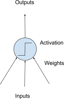
The building blocks for neural networks are artificial neurons.
These are simple computational units that have weighted input signals and produce an output signal using an activation function.
Model of a simple neuron
Neuron Weights
You may be familiar with linear regression, where the weights on the inputs are very much like the coefficients used in a regression equation.
Like linear regression, each neuron also has a bias which can be thought of as an input that always has the value 1.0, and it, too, must be weighted.
For example, a neuron may have two inputs, which require three weights—one for each input and one for the bias.
Weights are often initialized to small random values, such as values from 0 to 0.3, although more complex initialization schemes can be used.
Like linear regression, larger weights indicate increased complexity and fragility. Keeping weights in the network is desirable, and regularization techniques can be used.
Activation
The weighted inputs are summed and passed through an activation function, sometimes called a transfer function.
An activation function is a simple mapping of summed weighted input to the output of the neuron. It is called an activation function because it governs the threshold at which the neuron is activated and the strength of the output signal.
Historically, simple step activation functions were used when the summed input was above a threshold of 0.5, for example. Then the neuron would output a value of 1.0; otherwise, it would output a 0.0.
Traditionally, non-linear activation functions are used. This allows the network to combine the inputs in more complex ways and, in turn, provide a richer capability in the functions they can model. Non-linear functions like the logistic, also called the sigmoid function, were used to output a value between 0 and 1 with an s-shaped distribution. The hyperbolic tangent function, also called tanh, outputs the same distribution over the range -1 to +1.
More recently, the rectifier activation function has been shown to provide better results.
3. Networks of Neurons
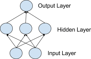
Neurons are arranged into networks of neurons.
A row of neurons is called a layer, and one network can have multiple layers. The architecture of the neurons in the network is often called the network topology.
Model of a simple network
Input or Visible Layers
The bottom layer that takes input from your dataset is called the visible layer because it is the exposed part of the network. Often a neural network is drawn with a visible layer with one neuron per input value or column in your dataset. These are not neurons as described above but simply pass the input value through to the next layer.
Hidden Layers
Layers after the input layer are called hidden layers because they are not directly exposed to the input. The simplest network structure is to have a single neuron in the hidden layer that directly outputs the value.
Given increases in computing power and efficient libraries, very deep neural networks can be constructed. Deep learning can refer to having many hidden layers in your neural network. They are deep because they would have been unimaginably slow to train historically but may take seconds or minutes to train using modern techniques and hardware.
Output Layer
The final hidden layer is called the output layer, and it is responsible for outputting a value or vector of values that correspond to the format required for the problem.
The choice of activation function in the output layer is strongly constrained by the type of problem that you are modeling. For example:
A regression problem may have a single output neuron, and the neuron may have no activation function.
A binary classification problem may have a single output neuron and use a sigmoid activation function to output a value between 0 and 1 to represent the probability of predicting a value for the class 1. This can be turned into a crisp class value by using a threshold of 0.5 and snap values less than the threshold to 0, otherwise to 1.
A multi-class classification problem may have multiple neurons in the output layer, one for each class (e.g., three neurons for the three classes in the famous iris flowers classification problem). In this case, a softmax activation function may be used to output a probability of the network predicting each of the class values. Selecting the output with the highest probability can be used to produce a crisp class classification value.
4. Training Networks
Once configured, the neural network needs to be trained on your dataset.
Data Preparation
You must first prepare your data for training on a neural network.
Data must be numerical, for example, real values. If you have categorical data, such as a sex attribute with the values “male” and “female,” you can convert it to a real-valued representation called one-hot encoding. This is where one new column is added for each class value (two columns in the case of sex of male and female), and a 0 or 1 is added for each row depending on the class value for that row.
This same one-hot encoding can be used on the output variable in classification problems with more than one class. This would create a binary vector from a single column that would be easy to directly compare to the output of the neuron in the network’s output layer. That, as described above, would output one value for each class.
Neural networks require the input to be scaled in a consistent way. You can rescale it to the range between 0 and 1, called normalization. Another popular technique is to standardize it so that the distribution of each column has a mean of zero and a standard deviation of 1.
Scaling also applies to image pixel data. Data such as words can be converted to integers, such as the popularity rank of the word in the dataset and other encoding techniques.
Stochastic Gradient Descent
The classical and still preferred training algorithm for neural networks is called stochastic gradient descent.
This is where one row of data is exposed to the network at a time as input. The network processes the input upward, activating neurons as it goes to finally produce an output value. This is called a forward pass on the network. It is the type of pass that is also used after the network is trained in order to make predictions on new data.
The output of the network is compared to the expected output, and an error is calculated. This error is then propagated back through the network, one layer at a time, and the weights are updated according to the amount they contributed to the error. This clever bit of math is called the backpropagation algorithm.
The process is repeated for all of the examples in your training data. One round of updating the network for the entire training dataset is called an epoch. A network may be trained for tens, hundreds, or many thousands of epochs.
Weight Updates
The weights in the network can be updated from the errors calculated for each training example, and this is called online learning. It can result in fast but also chaotic changes to the network.
Alternatively, the errors can be saved across all the training examples, and the network can be updated at the end. This is called batch learning and is often more stable.
Typically, because datasets are so large and because of computational efficiencies, the size of the batch, the number of examples the network is shown before an update, is often reduced to a small number, such as tens or hundreds of examples.
The amount that weights are updated is controlled by a configuration parameter called the learning rate. It is also called the step size and controls the step or change made to a network weight for a given error. Often small weight sizes are used, such as 0.1 or 0.01 or smaller.
The update equation can be complemented with additional configuration terms that you can set.
Momentum is a term that incorporates the properties from the previous weight update to allow the weights to continue to change in the same direction even when there is less error being calculated.
Learning Rate Decay is used to decrease the learning rate over epochs to allow the network to make large changes to the weights at the beginning and smaller fine-tuning changes later in the training schedule.
Prediction
Once a neural network has been trained, it can be used to make predictions.
You can make predictions on test or validation data in order to estimate the skill of the model on unseen data. You can also deploy it operationally and use it to make predictions continuously.
The network topology and the final set of weights are all you need to save from the model. Predictions are made by providing the input to the network and performing a forward-pass, allowing it to generate an output you can use as a prediction.
Need help with Deep Learning in Python?
Take my free 2-week email course and discover MLPs, CNNs and LSTMs (with code).
Click to sign-up now and also get a free PDF Ebook version of the course.
More Resources
There are decades of papers and books on the topic of artificial neural networks.
If you are new to the field, check out the following resources as further reading:
Thank you for this post @Jason. It’s very useful :D.
I have question please.
Since MLPs may hold many hidden layers so what is the difference between MLPs and DNN ? Or is them two face for same coin ?!
Dear Jason, great post and very clear explanations! I have two questions regarding data input. You mention that features such as “Gender” should be one-hot encoded, so you end up with two columns for gender instead of one. Then you mention that features need to be scaled or standardized. Do you need to do this scaling on the one-hot encoded categorical features? or only on the continuous features?
Thanks,
Dave
They provide a capability kind of like “levels of abstraction”. So-called “hierarchical learning”. That is the best we can say – we don’t have great theories for this stuff yet.
Thank you for the great article! I still have a question though. Every time I run a MLP in SPSS (not the best software i know, but it is the only thing available at the moment for me), I get different results. I know this has to do with the random number generation and that if i take the same initial value I get the same result. However, I was wondering if it is important to have multiple tries before you choose which model is best? Also, are the sum of squared errors a good measure to determine which one is best? How many times should you run the MLP before you can select the best one? And does it matter if the initial random number is chosen by me? Or not? I hope it aren’t too many questions! Thanks in advance.
For Day 03 on MLP:
A higher number of layers and neurons permits to increase the performance. Also, it appeared that the minimisation of ‘mae’ let’s achieve better performance than mnimization of ‘mse’ with ‘adam’ solver (not sure yet why).
# univariate mlp example
from numpy import array
from keras.models import Sequential
from keras.layers import Dense
from keras.layers import Dropout
# define dataset
X = np.array(input_df[‘x’].to_list())
y = np.array(input_df[‘y’].to_list())
Dear Jason,
Thank you for your post. If dataset has nominal variable about 80% , can I use Multi-Layer Perceptron Neural Networks ? Is it ok to use Multi-Layer Perceptron Neural Networks , if I change all nominal variable by dummy ?
I cannot see why it cannot. But how much impact you would see in the output is not guaranteed. You should experiment and judge whether this is a good idea.
Maybe these are unfair questions for a crash course, but I am curious.
1. What factors go into how many layers you choose for a network?
2. What factors go into how many neurons you choose per layer?
3. Since 2011 is it the state of practice to always use a rectifier activation function, or what factors would indicate a hyperbolic tangent or sigmoid?


This is a nice article but there are some typos that need to be corrected. Thank you for your time.
Thanks, what typos?
Thanks for the article, fairly easy to understand. I agree with the typos though, they are in your statement about epochs and somewhere else.
Thanks.
Great article! I‘m taking a class about Data Science and this article just made me understand this topic! Thx!
I’m glad it helped.
Hi Jason;
Are CNN, RNN and MLP supervised or unsupervised methods? Kindly mention which are used in each case.
Regards
They are all supervised.
this is a fantastic article, I am studying big data at uni and this made so much sense in a nutshell
Thanks, I’m glad it helped.
I would say my deep learning training is back propagated with Stochastic Gradient Descent after reading this article.
All my previous readings and training more clearer as I read this state of the art simple to comprehend article.
Thanks Dennis.
Thank you for this post @Jason. It’s very useful :D.
I have question please.
Since MLPs may hold many hidden layers so what is the difference between MLPs and DNN ? Or is them two face for same coin ?!
Oh i have just come to realize that MLPs is a type of architecture within DNN.
Thank you :).
A DNN is an MLP with lots of layers. Same thing really, just marketing.
Dear Jason, great post and very clear explanations! I have two questions regarding data input. You mention that features such as “Gender” should be one-hot encoded, so you end up with two columns for gender instead of one. Then you mention that features need to be scaled or standardized. Do you need to do this scaling on the one-hot encoded categorical features? or only on the continuous features?
Thanks,
Dave
One, the one hot encoded features can be used directly.
Hi
I have questions related to this topic
I started reading in blogs and scientific papers about deep learning and text classification methods
I’m struggling to distinguish between 1-DNN and 2-shallow neural networks as well as 3-MLP
what are the differences between them and which of them considered a deep learning algorithm or architecture?
They are all the same thing, deep just refers to more layers.
Dear Jason,
All methods talking about “Hidden Layers”, Please focus a little bit on it.
Kindly,
Ankit
Hidden layers are any layers that are not used for input or output of the model.
If hidden layers are ‘not’ used for input or output of the model, are they important while going for any model? if so, how?
Yes.
They provide a capability kind of like “levels of abstraction”. So-called “hierarchical learning”. That is the best we can say – we don’t have great theories for this stuff yet.
Dear Jason,
Thank you for the great article! I still have a question though. Every time I run a MLP in SPSS (not the best software i know, but it is the only thing available at the moment for me), I get different results. I know this has to do with the random number generation and that if i take the same initial value I get the same result. However, I was wondering if it is important to have multiple tries before you choose which model is best? Also, are the sum of squared errors a good measure to determine which one is best? How many times should you run the MLP before you can select the best one? And does it matter if the initial random number is chosen by me? Or not? I hope it aren’t too many questions! Thanks in advance.
Cheers!
Yes, this is to be expected:
https://machinelearningmastery.com/faq/single-faq/why-do-i-get-different-results-each-time-i-run-the-code
For Day 03 on MLP:
A higher number of layers and neurons permits to increase the performance. Also, it appeared that the minimisation of ‘mae’ let’s achieve better performance than mnimization of ‘mse’ with ‘adam’ solver (not sure yet why).
# univariate mlp example
from numpy import array
from keras.models import Sequential
from keras.layers import Dense
from keras.layers import Dropout
# define dataset
X = np.array(input_df[‘x’].to_list())
y = np.array(input_df[‘y’].to_list())
x_train = X[:300]
x_test = X[300:]
y_train = y[:300]
y_test = y[300:]
# define model
model = Sequential()
model.add(Dense(100, activation=’relu’, input_dim=4))
model.add(Dense(200, activation=’relu’, input_dim=4))
model.add(Dense(400, activation=’relu’, input_dim=4))
model.add(Dense(100, activation=’relu’, input_dim=4))
model.add(Dense(1))
model.compile(optimizer=’adam’, loss=’mae’)
# fit model
model.fit(X, y, epochs=3000, verbose=0)
# demonstrate prediction
yhat = model.predict(x_test, verbose=0)
y_pred = yhat.flatten()
print (“Mean absolute error: %2f”%metrics.mean_absolute_error(y_test, y_pred))
plt.plot(y_test)
plt.plot(y_pred, color=’r’)
>> Mean absolute error: 1.370448
Well done!
hi sir can you tell us about the multi-hot encoding?
Do you mean one-hot encoding?
If so, see this:
https://machinelearningmastery.com/one-hot-encoding-for-categorical-data/
Dear Jason,
Thank you for your post. If dataset has nominal variable about 80% , can I use Multi-Layer Perceptron Neural Networks ? Is it ok to use Multi-Layer Perceptron Neural Networks , if I change all nominal variable by dummy ?
Regards
I cannot see why it cannot. But how much impact you would see in the output is not guaranteed. You should experiment and judge whether this is a good idea.
Maybe these are unfair questions for a crash course, but I am curious.
1. What factors go into how many layers you choose for a network?
2. What factors go into how many neurons you choose per layer?
3. Since 2011 is it the state of practice to always use a rectifier activation function, or what factors would indicate a hyperbolic tangent or sigmoid?
Hi Mark,
The following resources may be of interest:
https://machinelearningmastery.com/how-to-configure-the-number-of-layers-and-nodes-in-a-neural-network/
https://machinelearningmastery.com/choose-an-activation-function-for-deep-learning/
Why is there no mention of labelling in the data preparation section?
Hi Nikhil…The following resource may be of interest:
https://machinelearningmastery.com/start-here/#dataprep
Thank you, Dr. Brownlee, for this helpful article.
I have a question.
I used this model to predict students’ performance (simple problem). What can I call it, and what is the limitation of this model?
python

def create_model():

    mlp = Sequential()

    mlp.add(Dense(5, input_dim=5, activation='relu'))

    mlp.add(Dense(1, activation='sigmoid'))

    mlp.compile(loss='binary_crossentropy', optimizer=Adam())

    return mlp
Hi Abdullah…What are the goals of your model? That is, what specifically are you predicting? That will allow us to better guide you.