A popular demonstration of the capability of deep learning techniques is object recognition in image data. The “hello world” of object recognition for machine learning and deep learning is the MNIST dataset for handwritten digit recognition. In this post, you will discover how to develop a deep learning model to achieve near state-of-the-art performance on the MNIST handwritten digit recognition task in PyTorch. After completing this chapter, you will know:
How to load the MNIST dataset using torchvision
How to develop and evaluate a baseline neural network model for the MNIST problem
How to implement and evaluate a simple Convolutional Neural Network for MNIST
How to implement a state-of-the-art deep learning model for MNIST
Kick-start your project with my book Deep Learning with PyTorch. It provides self-study tutorials with working code.
Let’s get started.
Handwritten Digit Recognition with LeNet5 Model in PyTorch Photo by Johnny Wong. Some rights reserved.
Overview
This post is divided into five parts; they are:
The MNIST Handwritten Digit Recognition Problem
Loading the MNIST Dataset in PyTorch
Baseline Model with Multilayer Perceptrons
Simple Convolutional Neural Network for MNIST
LeNet5 for MNIST
The MNIST Handwritten Digit Recognition Problem
The MNIST problem is a classic problem that can demonstrate the power of convolutional neural networks. The MNIST dataset was developed by Yann LeCun, Corinna Cortes, and Christopher Burges for evaluating machine learning models on the handwritten digit classification problem. The dataset was constructed from a number of scanned document datasets available from the National Institute of Standards and Technology (NIST). This is where the name for the dataset comes from, the Modified NIST or MNIST dataset.
Images of digits were taken from a variety of scanned documents, normalized in size, and centered. This makes it an excellent dataset for evaluating models, allowing the developer to focus on machine learning with minimal data cleaning or preparation required. Each image is a 28×28-pixel square (784 pixels total) in grayscale. A standard split of the dataset is used to evaluate and compare models, where 60,000 images are used to train a model, and a separate set of 10,000 images are used to test it.
To goal of this problem is to identify the digits on the image. There are ten digits (0 to 9) or ten classes to predict. The state-of-the-art prediction accuracy is at 99.8% level, achieved with large convolutional neural networks.
Want to Get Started With Deep Learning with PyTorch?
Take my free email crash course now (with sample code).
Click to sign-up and also get a free PDF Ebook version of the course.
Loading the MNIST Dataset in PyTorch
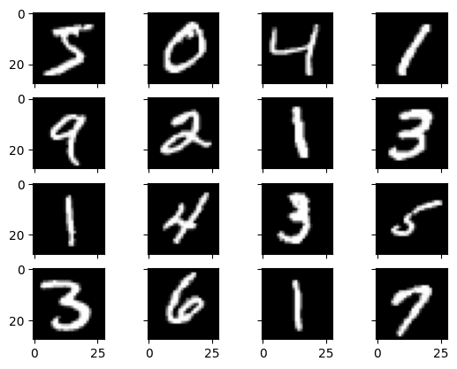
The torchvision library is a sister project of PyTorch that provide specialized functions for computer vision tasks. There is a function in torchvision that can download the MNIST dataset for use with PyTorch. The dataset is downloaded the first time this function is called and stored locally, so you don’t need to download again in the future. Below is a little script to download and visualize the first 16 images in the training subset of the MNIST dataset.
Do you really need a complex model like a convolutional neural network to get the best results with MNIST? You can get good results using a very simple neural network model with a single hidden layer. In this section, you will create a simple multilayer perceptron model that achieves accuracy of 99.81%. You will use this as a baseline for comparison to more complex convolutional neural network models. First, let’s check what the data looks like:
The training dataset is structured as a 3-dimensional array of instance, image height, and image width. For a multilayer perceptron model, you must reduce the images down into a vector of pixels. In this case, the 28×28-sized images will be 784 pixel input vectors. You can do this transform easily using the reshape() function.
The pixel values are grayscale between 0 and 255. It is almost always a good idea to perform some scaling of input values when using neural network models. Because the scale is well known and well behaved, you can very quickly normalize the pixel values to the range 0 and 1 by dividing each value by the maximum of 255.
In the following, you transform the dataset, convert to floating point, and normalize them by scaling floating point values and you can normalize them easily in the next step.
1
2
3
4
5
# each sample becomes a vector of values 0-1
X_train=train.data.reshape(-1,784).float()/255.0
y_train=train.targets
X_test=test.data.reshape(-1,784).float()/255.0
y_test=test.targets
The output targets y_train and y_test are labels in the form of integers from 0 to 9. This is a multiclass classification problem. You can convert these labels into one-hot encoding or keep them as integer labels like this case. You are going to use the cross entropy function to evaluate the model performance and the PyTorch implementation of cross entropy function can be applied on one-hot encoded targets or integer labeled targets.
You are now ready to create your simple neural network model. You will define your model in a PyTorch Module class.
1
2
3
4
5
6
7
8
9
10
11
classBaseline(nn.Module):
def __init__(self):
super().__init__()
self.layer1=nn.Linear(784,784)
self.act1=nn.ReLU()
self.layer2=nn.Linear(784,10)
def forward(self,x):
x=self.act1(self.layer1(x))
x=self.layer2(x)
returnx
The model is a simple neural network with one hidden layer with the same number of neurons as there are inputs (784). A rectifier activation function is used for the neurons in the hidden layer. The output of this model are logits, meaning they are real numbers which can be transformed into probability-like values using a softmax function. You do not apply the softmax function explicitly because the cross entropy function will do that for you.
You will use the stochastic gradient descent algorithm (with learning rate set to 0.01) to optimize this model. The training loop is as follows:
print("Epoch %d: model accuracy %.2f%%"%(epoch,acc*100))
Simple Convolutional Neural Network for MNIST
Now that you have seen how to use multilayer perceptron model to classify MNIST dataset. Let’s move on to try a convolutional neural network model. In this section, you will create a simple CNN for MNIST that demonstrates how to use all the aspects of a modern CNN implementation, including convolutional layers, pooling layers, and dropout layers.
In PyTorch, convolutional layers are supposed to work on images. Tensors for images should be the pixel values with the dimensions (sample, channel, height, width) but when you load images using libraries such as PIL, the pixels are usually presented as array of dimensions (height, width, channel). The conversion to a proper tensor format can be done using a transform from the torchvision library.
You need to use DataLoader because the transform is applied when you read the data from the DataLoader.
Next, define your neural network model. Convolutional neural networks are more complex than standard multilayer perceptrons, so you will start by using a simple structure that uses all the elements for state-of-the-art results. Below summarizes the network architecture.
The first hidden layer is a convolutional layer, nn.Conv2d(). The layer turns a grayscale image into 10 feature maps, with the filter size of 5×5 and a ReLU activation function. This is the input layer that expects images with the structure outlined above.
Next is a pooling layer that takes the max, nn.MaxPool2d(). It is configured with a pool size of 2×2 with stride 1. What it does is to take the maximum in a 2×2 pixel patch per channel and assign the value to the output pixel. The result is a 27×27-pixels feature map per channel.
The next layer is a regularization layer using dropout, nn.Dropout(). It is configured to randomly exclude 20% of neurons in the layer in order to reduce overfitting.
Next is a layer that converts the 2D matrix data to a vector, using nn.Flatten. There are 10 channels from its input and each channel’s feature map has size 27×27. This layer allows the output to be processed by standard, fully connected layers.
Next is a fully connected layer with 128 neurons. ReLU activation function is used.
Finally, the output layer has ten neurons for the ten classes. You can transform the output into probability-like predictions by applying a softmax function on it.
This model is trained using cross entropy loss and the Adam optimiztion algorithm. It is implemented as follows:
print("Epoch %d: model accuracy %.2f%%"%(epoch,acc*100))
LeNet5 for MNIST
The previous model has only one convolutional layer. Of course, you can add more to make a deeper model. One of the earliest demonstration of the effectiveness of convolutional layers in neural networks is the “LeNet5” model. This model is developed to solve the MNIST classification problem. It has three convolutional layers and two fully connected layer to make up five trainable layers in the model, as it is named.
At the time it was developed, using hyperbolic tangent function as activation is common. Hence it is used here. This model is implemented as follows:
Compare to the previous model, LeNet5 does not have Dropout layer (because Dropout layer was invented several years after LeNet5) and use average pooling instead of max pooling (i.e., for a patch of 2×2 pixels, it is taking average of the pixel values instead of taking the maximum). But the most notable characteristic of LeNet5 model is that it uses strides and paddings to reduce the image size from 28×28 pixel down to 1×1 pixel while increasing the number of channels from a one (grayscale) into 120.
Padding means to add pixels of value 0 at the border of the image to make it a bit larger. Without padding, the output of a convolutional layer will be smaller than its input. The stride parameter controls how much the filter should move to produce the next pixel in the output. Usually it is 1 to preserve the same size. If it is larger than 1, the output is a downsampling of the input. Hence you see in the LeNet5 model, stride 2 was used in the pooling layers to make, for example, a 28×28-pixel image into 14×14.
Training this model is same as training the previous convolutional network model, as follows:
In this post, you discovered the MNIST handwritten digit recognition problem and deep learning models developed in Python using the Keras library that are capable of achieving excellent results. Working through this chapter, you learned:
How to load the MNIST dataset in PyTorch with torchvision
How to convert the MNIST dataset into PyTorch tensors for consumption by a convolutional neural network
How to use PyTorch to create convolutional neural network models for MNIST
How to implement the LeNet5 model for MNIST classification
It provides self-study tutorials with hundreds of working code to turn you from a novice to expert. It equips you with tensor operation, training, evaluation, hyperparameter optimization,
and much more...
Kick-start your deep learning journey with hands-on exercises
One question for the data transform:
transform = torchvision.transforms.Compose([
torchvision.transforms.ToTensor(),
torchvision.transforms.Normalize((0,), (128,)),
])
The torchvision docs say that ToTensor transforms the image data from the range [0,255] to [0.0,1.0]. This is fine, but then applying Normalize((0,), (128,)) does not make sense, since this means divide by 128.
I’ve seen other recommendations of:
transform = torchvision.transforms.Compose([
torchvision.transforms.ToTensor(),
torchvision.transforms.Normalize((0.5,), (0.5,)),
])
Hi Michael…You’re absolutely correct in your observation, and the use of Normalize((0,), (128,)) in the provided transformation pipeline does not align with the usual intent of data normalization.
Here’s a detailed explanation:
### What ToTensor() Does
– The ToTensor() transformation converts image data from a PIL Image or NumPy array format in the range [0, 255] to a PyTorch tensor in the range [0.0, 1.0].
### What Normalize(mean, std) Does
– Normalize((mean,), (std,)) applies the transformation:
\[
\text{output} = \frac{\text{input} – \text{mean}}{\text{std}}
\]
Where:
– mean is the mean value to subtract.
– std is the standard deviation value by which to divide.
### Why Normalize((0,), (128,)) Doesn’t Make Sense
Since the data has already been scaled to [0.0, 1.0] by ToTensor(), applying Normalize((0,), (128,)) means dividing the scaled values by 128. This is likely a mistake or misunderstanding of the normalization process. Instead, you typically normalize the data to have a mean of 0.0 and a standard deviation of 1.0 by using appropriate values for mean and std.
### The Recommended Normalize((0.5,), (0.5,))
– Using Normalize((0.5,), (0.5,)) scales the data from [0.0, 1.0] to [-1.0, 1.0].
– First, subtracting 0.5 shifts the data to [-0.5, 0.5].
– Then, dividing by 0.5 scales it to [-1.0, 1.0].
This is a common practice for models that work well with input data in the range [-1, 1].
### Correct Transformation for LeNet-5
If you’re following a standard LeNet-5 implementation, it’s better to use: python
transform = torchvision.transforms.Compose([
torchvision.transforms.ToTensor(),
torchvision.transforms.Normalize((0.5,), (0.5,)), # Scales data to [-1, 1]
])
Alternatively, if you’re aiming for zero mean and unit variance normalization based on a dataset’s statistics (e.g., MNIST), you can use: python
transform = torchvision.transforms.Compose([
torchvision.transforms.ToTensor(),
torchvision.transforms.Normalize((0.1307,), (0.3081,)), # MNIST's mean and std
])
These statistics (mean=0.1307, std=0.3081) are computed from the MNIST dataset itself and are widely used in practice.
### Summary
– **Normalize((0,), (128,))** is incorrect unless there’s a specific reason to divide by 128 (unlikely here).
– Use **Normalize((0.5,), (0.5,))** for scaling to [-1, 1], or compute dataset-specific mean and std if zero-mean, unit-variance normalization is required.
– Choose the normalization based on the input expectations of the LeNet-5 implementation you’re using.


 with a BERT Model")


I think train should be False for the test dataset.
haha came here exactly to make the same observation
Thanks for the article.
One question for the data transform:
transform = torchvision.transforms.Compose([
torchvision.transforms.ToTensor(),
torchvision.transforms.Normalize((0,), (128,)),
])
The torchvision docs say that ToTensor transforms the image data from the range [0,255] to [0.0,1.0]. This is fine, but then applying Normalize((0,), (128,)) does not make sense, since this means divide by 128.
I’ve seen other recommendations of:
transform = torchvision.transforms.Compose([
torchvision.transforms.ToTensor(),
torchvision.transforms.Normalize((0.5,), (0.5,)),
])
which will scale the image data to [-1,1].
Hi Michael…You’re absolutely correct in your observation, and the use of
Normalize((0,), (128,))in the provided transformation pipeline does not align with the usual intent of data normalization.Here’s a detailed explanation:
### What
ToTensor()Does– The
ToTensor()transformation converts image data from a PIL Image or NumPy array format in the range[0, 255]to a PyTorch tensor in the range[0.0, 1.0].### What
Normalize(mean, std)Does–
Normalize((mean,), (std,))applies the transformation:\[
\text{output} = \frac{\text{input} – \text{mean}}{\text{std}}
\]
Where:
–
meanis the mean value to subtract.–
stdis the standard deviation value by which to divide.### Why
Normalize((0,), (128,))Doesn’t Make SenseSince the data has already been scaled to
[0.0, 1.0]byToTensor(), applyingNormalize((0,), (128,))means dividing the scaled values by128. This is likely a mistake or misunderstanding of the normalization process. Instead, you typically normalize the data to have a mean of0.0and a standard deviation of1.0by using appropriate values formeanandstd.### The Recommended
Normalize((0.5,), (0.5,))– Using
Normalize((0.5,), (0.5,))scales the data from[0.0, 1.0]to[-1.0, 1.0].– First, subtracting
0.5shifts the data to[-0.5, 0.5].– Then, dividing by
0.5scales it to[-1.0, 1.0].This is a common practice for models that work well with input data in the range
[-1, 1].### Correct Transformation for LeNet-5
If you’re following a standard LeNet-5 implementation, it’s better to use:
python

transform = torchvision.transforms.Compose([

    torchvision.transforms.ToTensor(),

    torchvision.transforms.Normalize((0.5,), (0.5,)),  # Scales data to [-1, 1]

])
Alternatively, if you’re aiming for zero mean and unit variance normalization based on a dataset’s statistics (e.g., MNIST), you can use:
python

transform = torchvision.transforms.Compose([

    torchvision.transforms.ToTensor(),

    torchvision.transforms.Normalize((0.1307,), (0.3081,)),  # MNIST's mean and std

])
These statistics (
mean=0.1307,std=0.3081) are computed from the MNIST dataset itself and are widely used in practice.### Summary
– **
Normalize((0,), (128,))** is incorrect unless there’s a specific reason to divide by 128 (unlikely here).– Use **
Normalize((0.5,), (0.5,))** for scaling to[-1, 1], or compute dataset-specificmeanandstdif zero-mean, unit-variance normalization is required.– Choose the normalization based on the input expectations of the LeNet-5 implementation you’re using.