In data analysis, SQL stands as a mighty tool, renowned for its robust capabilities in managing and querying databases. The pandas library in Python brings SQL-like functionalities to data scientists, enabling sophisticated data manipulation and analysis without the need for a traditional SQL database. In the following, you will apply SQL-like functions in Python to dissect and understand data.

Beyond SQL: Transforming Real Estate Data into Actionable Insights with Pandas
Photo by Lukas W. Some rights reserved.
Let’s get started.
Overview
This post is divided into three parts; they are:
- Exploring Data with Pandas’
DataFrame.query()Method - Aggregating and Grouping Data
- Mastering Row and Column Selection in Pandas
- Harnessing Pivot Table for In-Depth Housing Market Analysis
Exploring Data with Pandas’ DataFrame.query() Method
The DataFrame.query() method in pandas allows for the selection of rows based on a specified condition, akin to the SQL SELECT statement. Starting with the basics, you filter data based on single and multiple conditions, thereby laying the foundation for more complex data querying.
|
1 2 3 4 5 6 7 8 9 10 |
import pandas as pd import seaborn as sns import matplotlib.pyplot as plt # Load the dataset Ames = pd.read_csv('Ames.csv') # Simple querying: Select houses priced above $600,000 high_value_houses = Ames.query('SalePrice > 600000') print(high_value_houses) |
In the code above, you utilize the DataFrame.query() method from pandas to filter out houses priced above \$600,000, storing the result in a new DataFrame called high_value_houses. This method allows for concise and readable querying of the data based on a condition specified as a string. In this case, 'SalePrice > 600000'.
The resulting DataFrame below showcases the selected high-value properties. The query effectively narrows down the dataset to houses with a sale price exceeding \$600,000, showcasing merely 5 properties that meet this criterion. The filtered view provides a focused look at the upper echelon of the housing market in the Ames dataset, offering insights into the characteristics and locations of the highest-valued properties.
|
1 2 3 4 5 6 7 8 |
PID GrLivArea ... Latitude Longitude 65 528164060 2470 ... 42.058475 -93.656810 584 528150070 2364 ... 42.060462 -93.655516 1007 528351010 4316 ... 42.051982 -93.657450 1325 528320060 3627 ... 42.053228 -93.657649 1639 528110020 2674 ... 42.063049 -93.655918 [5 rows x 85 columns] |
In the next example below, let’s further explore the capabilities of the DataFrame.query() method to filter the Ames Housing dataset based on more specific criteria. The query selects houses that have more than 3 bedrooms (BedroomAbvGr > 3) and are priced below $300,000 (SalePrice < 300000). This combination of conditions is achieved using the logical AND operator (&), allowing you to apply multiple filters to the dataset simultaneously.
|
1 2 3 |
# Advanced querying: Select houses with more than 3 bedrooms and priced below $300,000 specific_houses = Ames.query('BedroomAbvGr > 3 & SalePrice < 300000') print(specific_houses) |
The result of this query is stored in a new DataFrame called specific_houses, which contains all the properties that satisfy both conditions. By printing specific_houses, you can examine the details of homes that are both relatively large (in terms of bedrooms) and affordable, targeting a specific segment of the housing market that could interest families looking for spacious living options within a certain budget range.
|
1 2 3 4 5 6 7 8 9 10 11 12 13 14 |
PID GrLivArea ... Latitude Longitude 5 908128060 1922 ... 42.018988 -93.671572 23 902326030 2640 ... 42.029358 -93.612289 33 903400180 1848 ... 42.029544 -93.627377 38 527327050 2030 ... 42.054506 -93.631560 40 528326110 2172 ... 42.055785 -93.651102 ... ... ... ... ... ... 2539 905101310 1768 ... 42.033393 -93.671295 2557 905107250 1440 ... 42.031349 -93.673578 2562 535101110 1584 ... 42.048256 -93.619860 2575 905402060 1733 ... 42.027669 -93.666138 2576 909275030 2002 ... NaN NaN [352 rows x 85 columns] |
The advanced query successfully identified a total of 352 houses from the Ames Housing dataset that meet the specified criteria: having more than 3 bedrooms and a sale price below \$300,000. This subset of properties highlights a significant portion of the market that offers spacious living options without breaking the budget, catering to families or individuals searching for affordable yet ample housing. To further explore the dynamics of this subset, let’s visualize the relationship between sale prices and ground living areas, with an additional layer indicating the number of bedrooms. This graphical representation will help you understand how living space and bedroom count influence the affordability and appeal of these homes within the specified criteria.
|
1 2 3 4 5 6 7 8 |
# Visualizing the advanced query results plt.figure(figsize=(10, 6)) sns.scatterplot(x='GrLivArea', y='SalePrice', hue='BedroomAbvGr', data=specific_houses, palette='viridis') plt.title('Sales Price vs. Ground Living Area') plt.xlabel('Ground Living Area (sqft)') plt.ylabel('Sales Price ($)') plt.legend(title='Bedrooms Above Ground') plt.show() |
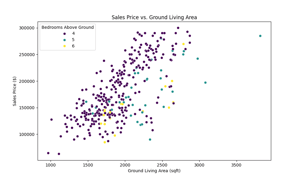
Scatter plot showing distribution of sales price related to the number of bedrooms and living area
The scatter plot above vividly demonstrates the nuanced interplay between sale price, living area, and bedroom count, underscoring the varied options available within this segment of the Ames housing market. It highlights how larger living spaces and additional bedrooms contribute to the property’s value, offering valuable insights for potential buyers and investors focusing on spacious yet affordable homes. This visual analysis not only makes the data more accessible but also underpins the practical utility of Pandas in uncovering key market trends.
Kick-start your project with my book The Beginner’s Guide to Data Science. It provides self-study tutorials with working code.
Aggregating and Grouping Data
Aggregation and grouping are pivotal in summarizing data insights. Building on the foundational querying techniques explored in the first part of your exploration, let’s delve deeper into the power of data aggregation and grouping in Python. Similar to SQL’s GROUP BY clause, pandas offers a robust groupby() method, enabling you to segment your data into subsets for detailed analysis. This next phase of your journey focuses on leveraging these capabilities to uncover hidden patterns and insights within the Ames Housing dataset. Specifically, you’ll examine the average sale prices of homes with more than three bedrooms, priced below \$300,000, across different neighborhoods. By aggregating this data, you aim to highlight the variability in housing affordability and inventory across the spatial canvas of Ames, Iowa.
|
1 2 3 4 5 6 7 8 9 10 11 12 13 14 15 |
# Advanced querying: Select houses with more than 3 bedrooms and priced below $300,000 specific_houses = Ames.query('BedroomAbvGr > 3 & SalePrice < 300000') # Group by neighborhood, then calculate the average and total sale price, and count the houses grouped_data = specific_houses.groupby('Neighborhood').agg({ 'SalePrice': ['mean', 'count'] }) # Renaming the columns for clarity grouped_data.columns = ['Average Sales Price', 'House Count'] # Round the average sale price to 2 decimal places grouped_data['Averages Sales Price'] = grouped_data['Average Sales Price'].round(2) print(grouped_data) |
|
1 2 3 4 5 6 7 8 9 10 11 12 13 14 15 16 17 18 19 20 21 22 23 24 |
Average Sales Price House Count Neighborhood BrDale 113700.00 1 BrkSide 154840.00 10 ClearCr 206756.31 13 CollgCr 233504.17 12 Crawfor 199946.68 19 Edwards 142372.41 29 Gilbert 222554.74 19 IDOTRR 146953.85 13 MeadowV 135966.67 3 Mitchel 152030.77 13 NAmes 158835.59 59 NPkVill 143000.00 1 NWAmes 203846.28 39 NoRidge 272222.22 18 NridgHt 275000.00 3 OldTown 142586.72 43 SWISU 147493.33 15 Sawyer 148375.00 16 SawyerW 217952.06 16 Somerst 247333.33 3 StoneBr 270000.00 1 Timber 247652.17 6 |
By employing Seaborn for visualization, let’s aim to create an intuitive and accessible representation of your aggregated data. You proceed with creating a bar plot that showcases the average sale price by neighborhood, complemented by annotations of house counts to illustrate both price and volume in a single, cohesive graph.
|
1 2 3 4 5 6 7 8 9 10 11 12 13 14 15 16 17 18 19 20 21 22 23 24 25 26 27 28 29 30 31 32 |
# Ensure 'Neighborhood' is a column (reset index if it was the index) grouped_data_reset = grouped_data.reset_index().sort_values(by='Average Sales Price') # Set the aesthetic style of the plots sns.set_theme(style="whitegrid") # Create the bar plot plt.figure(figsize=(12, 8)) barplot = sns.barplot( x='Neighborhood', y='Average Sales Price', data=grouped_data_reset, palette="coolwarm", hue='Neighborhood', legend=False, errorbar=None # Removes the confidence interval bars ) # Rotate the x-axis labels for better readability plt.xticks(rotation=45) # Annotate each bar with the house count, using enumerate to access the index for positioning for index, value in enumerate(grouped_data_reset['Average Sales Price']): house_count = grouped_data_reset.loc[index, 'House Count'] plt.text(index, value, f'{house_count}', ha='center', va='bottom') plt.title('Average Sales Price by Neighborhood', fontsize=18) plt.xlabel('Neighborhood') plt.ylabel('Average Sales Price ($)') plt.tight_layout() # Adjust the layout plt.show() |
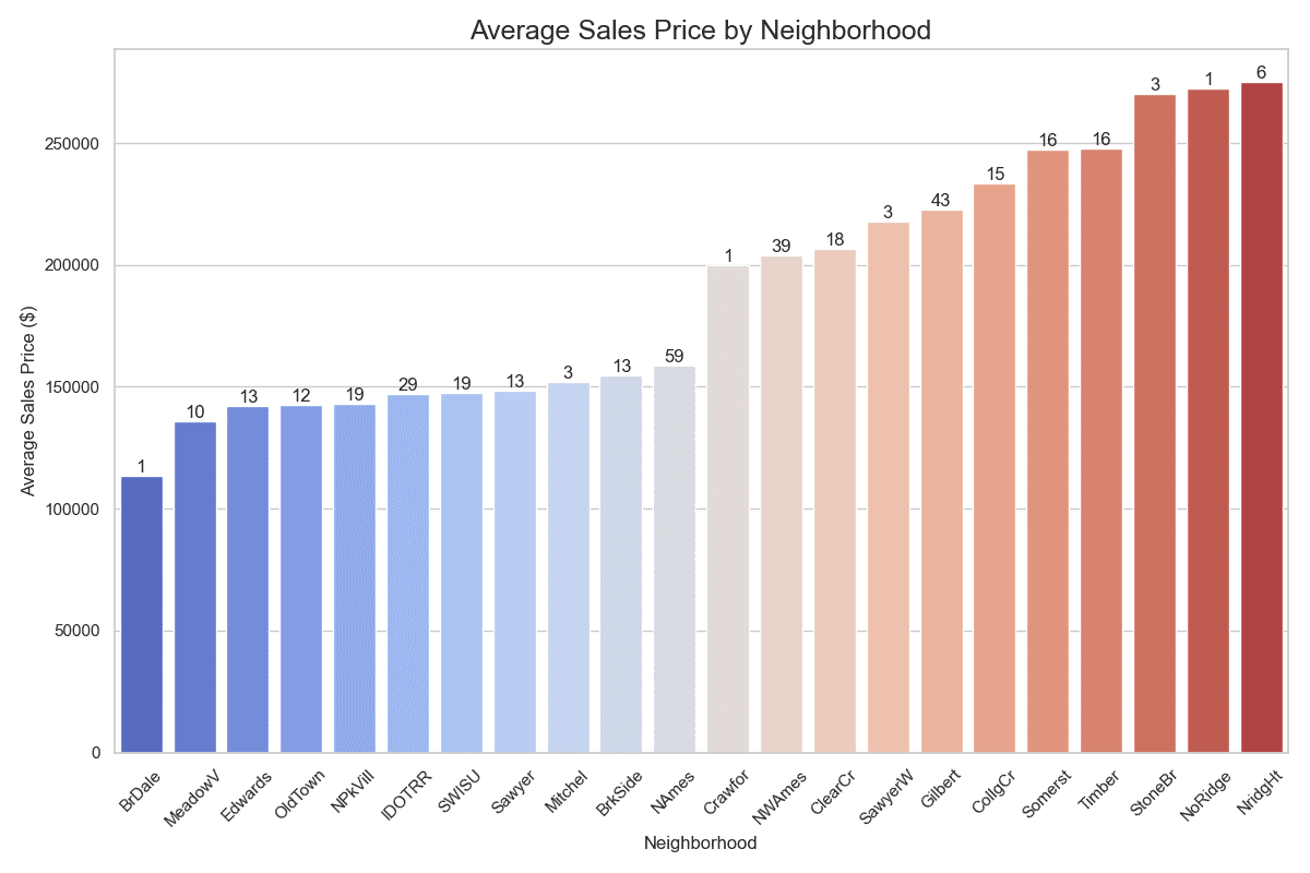
Comparing neighborhoods by ascending average sales price
The analysis and subsequent visualization underscore the significant variability in both the affordability and availability of homes that meet specific criteria—more than three bedrooms and priced below \$300,000—across Ames, Iowa. This not only demonstrates the practical application of SQL-like functions in Python for real-world data analysis but also provides valuable insights into the dynamics of local real estate markets.
Mastering Row and Column Selection in Pandas
Selecting specific subsets of data from DataFrames is a frequent necessity. Two powerful methods at your disposal are DataFrame.loc[] and DataFrame.iloc[]. Both serve similar purposes—to select data—but they differ in how they reference the rows and columns.
Understanding The DataFrame.loc[] Method
DataFrame.loc[] is a label-based data selection method, meaning you use the labels of rows and columns to select the data. It’s highly intuitive for selecting data based on column names and row indexes when you know the specific labels you’re interested in.
Syntax: DataFrame.loc[row_label, column_label]
Goal: Let’s select all houses with more than 3 bedrooms, priced below \$300,000, in specific neighborhoods known for their higher average sale prices (based on your earlier findings), and display their ‘Neighborhood’, ‘SalePrice’ and ‘GrLivArea’.
|
1 2 3 4 5 6 7 8 9 10 |
# Assuming 'high_value_neighborhoods' is a list of neighborhoods with higher average sale prices high_value_neighborhoods = ['NridgHt', 'NoRidge', 'StoneBr'] # Use df.loc[] to select houses based on your conditions and only in high-value neighborhoods high_value_houses_specific = Ames.loc[(Ames['BedroomAbvGr'] > 3) & (Ames['SalePrice'] < 300000) & (Ames['Neighborhood'].isin(high_value_neighborhoods)), ['Neighborhood', 'SalePrice', 'GrLivArea']] print(high_value_houses_specific.head()) |
|
1 2 3 4 5 6 |
Neighborhood SalePrice GrLivArea 40 NoRidge 291000 2172 162 NoRidge 285000 2225 460 NridgHt 250000 2088 468 NoRidge 268000 2295 490 NoRidge 260000 2417 |
Understanding The DataFrame.iloc[] Method
In contrast, DataFrame.iloc[] is an integer-location based indexing method. This means you use integers to specify the rows and columns you want to select. It’s particularly useful to access data by its position in the DataFrame.
Syntax: DataFrame.iloc[row_position, column_position]
Goal: The next focus is to uncover affordable housing options within the Ames dataset that do not compromise on space, specifically targeting homes with at least 3 bedrooms above grade and priced below \$300,000 outside of high-value neighborhoods.
|
1 2 3 4 5 6 7 8 9 10 11 12 13 14 |
# Filter for houses not in the 'high_value_neighborhoods', # with at least 3 bedrooms above grade, and priced below $300,000 low_value_spacious_houses = Ames.loc[(~Ames['Neighborhood'].isin(high_value_neighborhoods)) & (Ames['BedroomAbvGr'] >= 3) & (Ames['SalePrice'] < 300000)] # Sort these houses by 'SalePrice' to highlight the lower end explicitly low_value_spacious_houses_sorted = low_value_spacious_houses.sort_values(by='SalePrice').reset_index(drop=True) # Using df.iloc to select and print the first 5 observations of such low-value houses low_value_spacious_first_5 = low_value_spacious_houses_sorted.iloc[:5, :] # Print only relevant columns to match the earlier high-value example: 'Neighborhood', 'SalePrice', 'GrLivArea' print(low_value_spacious_first_5[['Neighborhood', 'SalePrice', 'GrLivArea']]) |
|
1 2 3 4 5 6 |
Neighborhood SalePrice GrLivArea 0 IDOTRR 40000 1317 1 IDOTRR 50000 1484 2 IDOTRR 55000 1092 3 Sawyer 62383 864 4 Edwards 63000 1112 |
In your exploration of DataFrame.loc[] and DataFrame.iloc[], you’ve uncovered the capabilities of pandas for row and column selection, demonstrating the flexibility and power of these methods in data analysis. Through practical examples from the Ames Housing dataset, you’ve seen how DataFrame.loc[] allows for intuitive, label-based selection, ideal for targeting specific data based on known labels. Conversely, DataFrame.iloc[] provides a precise way to access data by its integer location, offering an essential tool for positional selection, especially useful in scenarios requiring a focus on data segments or samples. Whether filtering for high-value properties in select neighborhoods or identifying entry-level homes in the broader market, mastering these selection techniques enriches your data science toolkit, enabling more targeted and insightful data exploration.
Want to Get Started With Beginner's Guide to Data Science?
Take my free email crash course now (with sample code).
Click to sign-up and also get a free PDF Ebook version of the course.
Harnessing Pivot Tables for In-depth Housing Market Analysis
As you venture further into the depths of the Ames Housing dataset, your analytical journey introduces you to the potent capabilities of pivot tables within pandas. Pivot tables serve as an invaluable tool for summarizing, analyzing, and presenting complex data in an easily digestible format. This technique allows you to cross-tabulate and segment data to uncover patterns and insights that might otherwise remain hidden. In this section, you’ll leverage pivot tables to dissect the housing market more intricately, focusing on the interplay between neighborhood characteristics, the number of bedrooms, and sale prices.
To set the stage for your pivot table analysis, you filter the dataset for homes priced below \$300,000 and with at least one bedroom above grade. This criterion focuses on more affordable housing options, ensuring your analysis remains relevant to a broader audience. You then proceed to construct a pivot table that segments the average sale price by neighborhood and bedroom count, aiming to uncover patterns that dictate housing affordability and preference within Ames.
|
1 2 3 4 5 6 7 8 9 10 11 12 13 14 15 16 17 18 19 |
# Import an additional library import numpy as np # Filter for houses priced below $300,000 and with at least 1 bedroom above grade affordable_houses = Ames.query('SalePrice < 300000 & BedroomAbvGr > 0') # Create a pivot table to analyze average sale price by neighborhood and number of bedrooms pivot_table = affordable_houses.pivot_table(values='SalePrice', index='Neighborhood', columns='BedroomAbvGr', aggfunc='mean').round(2) # Fill missing values with 0 for better readability and to indicate no data for that segment pivot_table = pivot_table.fillna(0) # Adjust pandas display options to ensure all columns are shown pd.set_option('display.max_columns', None) print(pivot_table) |
Let’s take a quick view of the pivot table before we discuss some insights.
|
1 2 3 4 5 6 7 8 9 10 11 12 13 14 15 16 17 18 19 20 21 22 23 24 25 26 27 28 29 30 |
BedroomAbvGr 1 2 3 4 5 6 Neighborhood Blmngtn 178450.00 197931.19 0.00 0.00 0.00 0.00 Blueste 192500.00 128557.14 151000.00 0.00 0.00 0.00 BrDale 0.00 99700.00 111946.43 113700.00 0.00 0.00 BrkSide 77583.33 108007.89 140058.67 148211.11 214500.00 0.00 ClearCr 212250.00 220237.50 190136.36 209883.20 196333.33 0.00 CollgCr 154890.00 181650.00 196650.98 233504.17 0.00 0.00 Crawfor 289000.00 166345.00 193433.75 198763.94 210000.00 0.00 Edwards 59500.00 117286.27 134660.65 137332.00 191866.67 119900.00 Gilbert 0.00 172000.00 182178.30 223585.56 204000.00 0.00 Greens 193531.25 0.00 0.00 0.00 0.00 0.00 GrnHill 0.00 230000.00 0.00 0.00 0.00 0.00 IDOTRR 67378.00 93503.57 111681.13 144081.82 162750.00 0.00 Landmrk 0.00 0.00 137000.00 0.00 0.00 0.00 MeadowV 82128.57 105500.00 94382.00 128250.00 151400.00 0.00 Mitchel 176750.00 150366.67 168759.09 149581.82 165500.00 0.00 NAmes 139500.00 133098.93 146260.96 159065.22 180360.00 144062.50 NPkVill 0.00 134555.00 146163.64 143000.00 0.00 0.00 NWAmes 0.00 177765.00 183317.12 201165.00 253450.00 0.00 NoRidge 0.00 262000.00 259436.67 272222.22 0.00 0.00 NridgHt 211700.00 215458.55 264852.71 275000.00 0.00 0.00 OldTown 83333.33 105564.32 136843.57 136350.91 167050.00 97500.00 SWISU 60000.00 121044.44 132257.88 143444.44 158500.00 148633.33 Sawyer 185000.00 124694.23 138583.77 148884.62 0.00 146166.67 SawyerW 216000.00 156147.41 185192.14 211315.00 0.00 237863.25 Somerst 205216.67 191070.18 225570.39 247333.33 0.00 0.00 StoneBr 223966.67 211468.75 233750.00 270000.00 0.00 0.00 Timber 0.00 217263.64 200536.04 241202.60 279900.00 0.00 Veenker 247566.67 245150.00 214090.91 0.00 0.00 0.00 |
The pivot table above provides a comprehensive snapshot of how the average sale price varies across neighborhoods with the inclusion of different bedroom counts. This analysis reveals several key insights:
- Affordability by Neighborhood: You can see at a glance which neighborhoods offer the most affordable options for homes with specific bedroom counts, aiding in targeted home searches.
- Impact of Bedrooms on Price: The table highlights how the number of bedrooms influences sale prices within each neighborhood, offering a gauge of the premium placed on larger homes.
- Market Gaps and Opportunities: Areas with zero values indicate a lack of homes meeting certain criteria, signaling potential market gaps or opportunities for developers and investors.
By leveraging pivot tables for this analysis, you’ve managed to distill complex relationships within the Ames housing market into a format that’s both accessible and informative. This process not only showcases the powerful synergy between pandas and SQL-like analysis techniques but also emphasizes the importance of sophisticated data manipulation tools in uncovering actionable insights within real estate markets. As insightful as pivot tables are, their true potential is unleashed when combined with visual analysis.
To further illuminate your findings and make them more intuitive, you’ll transition from numerical analysis to visual representation. A heatmap is an excellent tool for this purpose, especially when dealing with multidimensional data like this. However, to enhance the clarity of your heatmap and direct attention towards actionable data, you will employ a custom color scheme that distinctly highlights non-existent combinations of neighborhood and bedroom counts.
|
1 2 3 4 5 6 7 8 9 10 11 12 13 14 15 16 17 18 19 20 21 22 23 24 25 26 27 28 |
# Import an additional library import matplotlib.colors # Create a custom color map cmap = matplotlib.colors.LinearSegmentedColormap.from_list("", ["red", "yellow", "green"]) # Mask for "zero" values to be colored with a different shade mask = pivot_table == 0 # Set the size of the plot plt.figure(figsize=(14, 10)) # Create a heatmap with the mask sns.heatmap(pivot_table, cmap=cmap, annot=True, fmt=".0f", linewidths=.5, mask=mask, cbar_kws={'label': 'Average Sales Price ($)'}) # Adding title and labels for clarity plt.title('Average Sales Price by Neighborhood and Number of Bedrooms', fontsize=16) plt.xlabel('Number of Bedrooms Above Grade', fontsize=12) plt.ylabel('Neighborhood', fontsize=12) # Display the heatmap plt.show() |
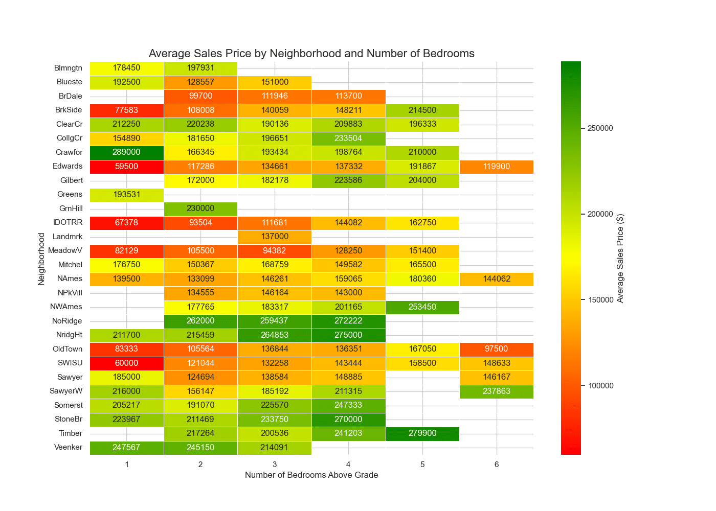
Heatmap showing the average sales price by neighborhood
The heatmap vividly illustrates the distribution of average sale prices across neighborhoods, segmented by the number of bedrooms. This color-coded visual aid makes it immediately apparent which areas of Ames offer the most affordable housing options for families of various sizes. Moreover, the distinct shading for zero values—indicating combinations of neighborhoods and bedroom counts that do not exist—is a critical tool for market analysis. It highlights gaps in the market where demand might exist, but supply does not, offering valuable insights for developers and investors alike. Remarkably, your analysis also highlights that homes with 6 bedrooms in the “Old Town” neighborhood are listed at below \$100,000. This discovery points to exceptional value for larger families or investors looking for properties with high bedroom counts at affordable price points.
Through this visual exploration, you’ve not only enhanced your understanding of the housing market’s dynamics but also demonstrated the indispensable role of advanced data visualization in real estate analysis. The pivot table, complemented by the heatmap, exemplifies how sophisticated data manipulation and visualization techniques can reveal informative insights into the housing sector.
Further Reading
This section provides more resources on the topic if you want to go deeper.
Python Documentation
- Pandas’
DataFrame.query()Method - Pandas’
DataFrame.groupby()Method - Pandas’
DataFrame.loc[]Method - Pandas’
DataFrame.iloc[]Method - Pandas’
DataFrame.pivot_table()Method
Resources
Summary
This comprehensive journey through the Ames Housing dataset underscores the versatility and strength of pandas for conducting sophisticated data analysis, often achieving or exceeding what’s possible with SQL in an environment that doesn’t rely on traditional databases. From pinpointing detailed housing market trends to identifying unique investment opportunities, you’ve showcased a range of techniques that equip analysts with the tools needed for deep data exploration. Specifically, you learned how to:
- Leverage the
DataFrame.query()for data selection akin to SQL’sSELECTstatement. - Use
DataFrame.groupby()for aggregating and summarizing data, similar to SQL’sGROUP BY. - Apply advanced data manipulation techniques like
DataFrame.loc[],DataFrame.iloc[], andDataFrame.pivot_table()for deeper analysis.
Do you have any questions? Please ask your questions in the comments below, and I will do my best to answer.
Get Started on The Beginner's Guide to Data Science!
Learn the mindset to become successful in data science projects
...using only minimal math and statistics, acquire your skill through short examples in Python
Discover how in my new Ebook:
The Beginner's Guide to Data Science
It provides self-study tutorials with all working code in Python to turn you from a novice to an expert. It shows you how to find outliers, confirm the normality of data, find correlated features, handle skewness, check hypotheses, and much more...all to support you in creating a narrative from a dataset.


No comments yet.