The 2025 Machine Learning Toolbox: Top Libraries and Tools for Practitioners

The 2025 Machine Learning Toolbox: Top Libraries and Tools for Practitioners
Image by Author | Ideogram

2024 was the year machine learning (ML) and artificial intelligence (AI) went mainstream, affecting peoples’ lives in ways they never before could have. With the introduction of large language model (LLM) products in recent years such as ChatGPT, companies are racing to apply the power of ML, AI, and LLMs to their businesses.

In 2025, many emerging trends within the ML world will continue to be front and center in many business operations. Trends such as agents, generative AI, explainability, and more will continue to shape our future. This means we should be able to keep up with these trends.

This article will explore the top machine learning libraries and tools for practitioners in 2025. The toolbox outlined in this article will become your baseline for navigating emerging trends.

LangChain

The first library you need to know in 2025 is LangChain, including their extended family of products.

In the era of LLM applications, the ability to quickly build and deploy applications has become more important than ever. As a library, LangChain provides a framework to streamline the development of LLM-powered applications, making the process more efficient and scalable.

LangChain provides many tools that simplify the LLM application development process using various components such as chains, prompt templates, and more. The framework also supports integration with various LLM providers such as OpenAI, Gemini, and Hugging Face.

However, an even better reason for adopting LangChain is its active development and strong open source community. With this support, LangChain can be the perfect tool for building your LLM application.

LangChain also stands out because of the tools within its family, namely LangGraph and LangSmith. LangGraph is built on top of LangChain to manage agentic workflow using a graph-based approach. Meanwhile, LangSmith complements LangChain and LangGraph by providing tools for the application lifecycle, such as monitoring, testing, and optimization.

Let’s try out the LangChain library. First, we will install the library:

We will also use the Gemini model as the LLM engine, so you will have to acquire an API key. Next, we set up the library and LLM for our application:

Lastly, we set up the prompt template and the sequence to provide a response from the LLM.

We already set up the LLM applications with just a few lines above. Of course, this implementation is still very simple and needs more consideration and additional tweaks to be stable in production, but it should demonstrate how powerful LangChain can be with just a few lines of code.

JAX

If you are a data scientist or have previously developed machine learning models with Python, you may be familiar with the NumPy library. JAX is a Python library that provides numerical computational like NymPy but with powerful capabilities for machine learning research and implementation.

The Google team develops JAX to allow high-performance computation and to provide features such as automatic differentiation, vectorization, or just-in-time (JIT) compilation. The features are designed to achieve intensive computation with ease. JAX has been used in many machine learning applications. The module provides many APIs suitable for high-performance simulation and experiments.

Let’s check out JAX with the following code. First, we install.

Now we can try out the JAX computational functions. For example, we will compute the gradient from the given function.

And the output from the above code would be:

We can also vectorize the function and apply it to the array.

And the output:

You can check the documentation to learn more about the library. It provides extensive material that you can explore to understand how it works.

Fastai

 
The next tool is Fastai, which provides a fast implementation of deep learning techniques and helper functionality. The library is designed to simplify neural network training using high-level components that allow practitioners to achieve great results with minimal code.

The Fastai library is built on top of the PyTorch library, so much of the PyTorch power and flexibility is available from within. However, Fastai provides a much easier way for users to build models as the library abstracts a lot of the complex code into a simple API. Still, Fastai can be used to create custom models as the library also provides low-level components.

Fastai supports many tasks, such as computer vision, tabular data, natural language processing, etc. Depending on your needs, you can use the code as it is or progressively increase the complexity as required.

Let’s try to use the library to understand it better.

First, we need to install the Fastai library. I recommend using Miniconda, but you can also use other installation methods. The PyTorch library is also important, as it is a prerequisite.

You can install the library via pip using the following code:

Once you install the Fastai library we can use it to build a deep learning model for ourselves. For example, we will create a sentiment text classifier model using data from Kaggle.

Let’s prepare the text data and all the required libraries for the tutorial.

Next, we will perform model fine-tuning using Fastai. Before building the model classifier, let’s look at how the library can assist with fine-tuning tasks.

We must prepare the dataset in a format that Fastai could use using the following code.

This tutorial will use and fine-tune the AWD-LSTM architecture, as shown in the code below. You can tweak the learning rate and the epoch number if you wish as well.

The code above will fine-tune the language model object and result in the model object being saved in your directory. You now have your base language model. Let’s see how to fine-tune the pre-trained language model for the text classifier.

We will prepare the dataset once more but with a tweak this time.

You can see that I set the text_vocab parameter using vocabulary from the dataset used for fine-tuning to maintain consistency, and set the is_lm to False to ensure the model knows it is to be used for classification tasks.

Then, we train the classifier with the following code.

We have now finished developing our model classifier and obtained the model. We can see how the model performs against the test dataset using the code below.

You can also test the classifier model with the following code.

Output:

That’s how easily you could train your model with Fastai. You can use the documentation to explore other use cases.

IntepretML

With explainability and ethics becoming increasingly prominent trends in 2025, we need to understand why our machine learning models produce the outputs they do. This is why IntepretML should be in your machine learning toolbox.

InterpretML is a Python library developed by Microsoft that enables users to train interpretable machine learning models, such as the explainable boosting machine (EBM), and to explain black box models using techniques like SHAP and LIME. Additionally, it offers an interactive visualization dashboard for in-depth exploration of model explanations.

Let’s see how it works using the notebook example. First, we need to install the IntepretML library.

Next, we will prepare the sample dataset by preprocessing it and using an EBM model to train the classifier.

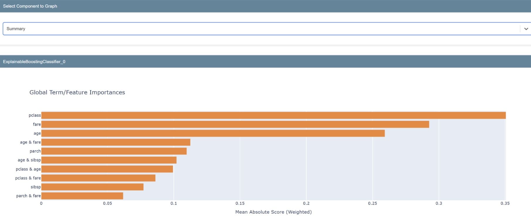
Once the model is ready, we can examine the library’s explainability. We will examine the global explainability which is the model’s overall explainability.

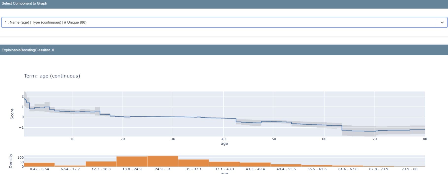
The summary will produce a graph showing the importance of our model’s features. A single feature can also be examined to understand its prediction distribution.

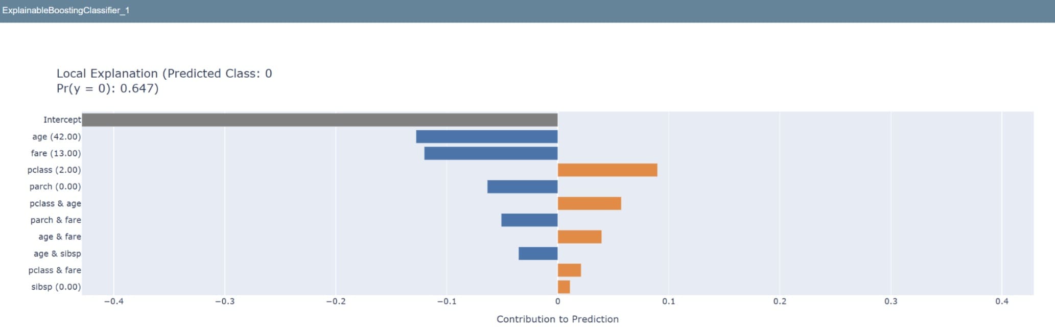
If we want to see how the model predicts singular data, the following code allows us to do so.

Try using this library to help gain the trust of the stakeholders. Explainability is how non-technical people will understand what happens within your model.

TokenSHAP

SHAP is a technique that we use to have explainability from our model for the global and local levels using the Shapley value. TokenSHAP uses the SHAP technique to interpret the LLM using the Monte Carlo Shapley Value Estimation technique. The library will estimate individual tokens’ Shapley values and explain how each token contributes to the model decision.

Let’s try out the library by first installing it.

Then, we will use TokenSHAP to understand how the prompt contributes to the Gemini model result. To do that, we will develop a custom class that TokenSHAP can process.

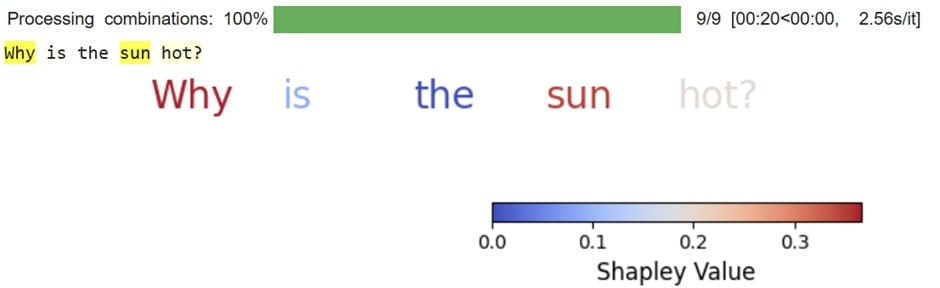
When the model is ready, we will use it to perform a SHAP analysis on the LLMs.

The result is an individual token colored based on its Shapley Value. The higher the Shapley value, the more influential that token is to the model response. For example, the words why and sun are much more important than the word the when providing output.

Using the code below, you can also get the exact Shapley value for each token.

Output:

Try utilizing TokenSHAP to understand why your LLM provides certain output and which tokens plays the greater roles in the process.

Conclusion

This article explored a suite of powerful tools shaping machine learning in 2025 — from the rapid application development enabled by the LangChain family to the high-performance numerical capabilities of JAX. We also looked into Fastai’s streamlined deep learning framework, the interpretability advantages offered by InterpretML, and the token-level insights provided by TokenSHAP. Each of these libraries not only exemplifies emerging trends like generative AI and enhanced model explainability but also equips you with practical, hands-on approaches for tackling complex challenges in today’s data-driven landscape.

Moving forward, harnessing these tools will empower you to build robust, scalable, and transparent ML solutions. Embrace these innovations to refine your workflows and drive impactful results, confident that you are well-prepared to lead in the evolving world of machine learning and artificial intelligence.

I hope this has helped!