Loss Functions in PyTorch Models

The loss metric is very important for neural networks. As all machine learning models are one optimization problem or another, the loss is the objective function to minimize. In neural networks, the optimization is done with gradient descent and backpropagation. But what are loss functions, and how are they affecting your neural networks?

In this chapter, you will learn what loss functions are and delve into some commonly used loss functions and how you can apply them to your neural networks. After reading this chapter, you will learn:

• What are loss functions, and their role in training neural network models
• Common loss functions for regression and classification problems
• How to use loss functions in your PyTorch model

Kick-start your project with my book Deep Learning with PyTorch. It provides self-study tutorials with working code.

Loss Functions in PyTorch Models.
Photo by Hans Vivek. Some rights reserved.

Overview

This post is divided into four sections; they are:

• What Are Loss Functions?
• Loss Functions for Regression
• Loss Functions for Classification
• Custom Loss Function in PyTorch

What Are Loss Functions?

In neural networks, loss functions help optimize the performance of the model. They are usually used to measure some penalty that the model incurs on its predictions, such as the deviation of the prediction away from the ground truth label. Loss functions are usually differentiable across their domain (but it is allowed that the gradient is undefined only for very specific points, such as $x=0$, which is basically ignored in practice). In the training loop, they are differentiated with respect to parameters, and these gradients are used for your backpropagation and gradient descent steps to optimize your model on the training set.

Loss functions are also slightly different from metrics. While loss functions can tell you the performance of our model, they might not be of direct interest or easily explainable by humans. This is where metrics come in. Metrics such as accuracy are much more useful for humans to understand the performance of a neural network even though they might not be good choices for loss functions since they might not be differentiable.

In the following, let’s explore some common loss functions, for regression problems and for classification problems.

Loss Functions for Regression

In regression problems, the model is to predict a value in a continuous range. Too good to be true that your model can predict the exact value all the time, but it is good enough if the value is close enough. Therefore, you need a loss function to measure how close it is. The farther away from the exact value, the more the loss is your prediction.

One simple function is just to measure the difference between the prediction and the target value. You do not care the value is greater than or less than the target value in finding the difference. Hence, in mathematics, we find $\dfrac{1}{m}\sum_{i=1}^m \vert \hat{y}_i – y_i\vert$ with $m$ the number of training examples whereas $y_i$ and $\hat{y}_i$ are the target and predicted values, respectively, averaged over all training examples. This is the mean absolute error (MAE).

The MAE is never negative and would be zero only if the prediction matched the ground truth perfectly. It is an intuitive loss function and might also be used as one of your metrics, specifically for regression problems, since you want to minimize the error in your predictions.

However, absolute value is not differentiable at 0. It is not really a problem because you rarely hitting that value. But sometimes people would prefer to use mean square error (MSE) instead. MSE equals to $\dfrac{1}{m}\sum_{i=1}^m (\hat{y}_i – y_i)^2$, which is similar to MAE but use square function in place of absolute value.

It also measures the deviation of the predicted value from the target value. However, the MSE squares this difference (always non-negative since squares of real numbers are always non-negative), which gives it slightly different properties. One property is that the mean squared error favors a large number of small errors over a small number of large errors, which leads to models with fewer outliers or at least outliers that are less severe than models trained with a MAE. This is because a large error would have a significantly larger impact on the error and, consequently, the gradient of the error when compared to a small error.

Let’s look at what the mean absolute error and mean square error loss function looks like graphically:

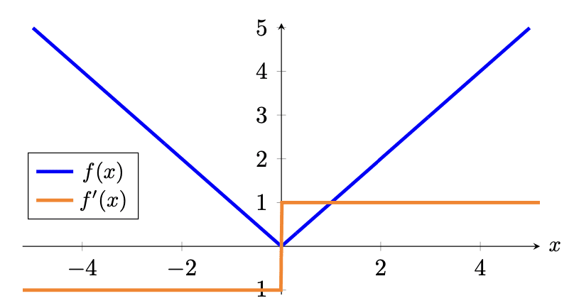
Mean absolute error loss function (blue) and gradient (orange)

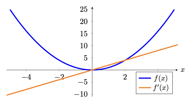
Mean square error loss function (blue) and gradient (orange)

Similar to activation functions, you might also be interested in what the gradient of the loss function looks like since you are using the gradient later to do backpropagation to train your model’s parameters. You should see that in MSE, larger errors would lead to a larger magnitude for the gradient and a larger loss. Hence, for example, two training examples that deviate from their ground truths by 1 unit would lead to a loss of 2, while a single training example that deviates from its ground truth by 2 units would lead to a loss of 4, hence having a larger impact. This is not the case in MAE.

In PyTorch, you can create MAE and MSE as loss functions using nn.L1Loss() and nn.MSELoss() respectively. It is named as L1 because the computation of MAE is also called the L1-norm in mathematics. Below is an example of computing the MAE and MSE between two vectors:

You should get

MAE is 2.0 because $\frac{1}{2}[\vert 0-1\vert + \vert 3-0\vert]=\frac{1}{2}(1+3)=2$ whereas MSE is 5.0 because $\frac{1}{2}[(0-1)^2 + (3-0)^2]=\frac{1}{2}(1+9)=5$. Notice that in MSE, the second example with a predicted value of 3 and actual value of 0 contributes 90% of the error under the mean squared error vs. 75% under the mean absolute error.

Sometimes, you may see people use root mean squared error (RMSE) as a metric. This will take the square root of MSE. From the perspective of a loss function, MSE and RMSE are equivalent. But from the perspective of the value, the RMSE is in the same unit as the predicted values. If your prediction is money in dollars, both MAE and RMSE give you how much your prediction is away from the true value in dollars in average. But MSE is in unit of squared dollars, which its physical meaning is not intuitive.

Loss Functions for Classification

For classification problems, there is a small, discrete set of numbers that the output could take. Furthermore, the number used to label-encode the classes is arbitrary and with no semantic meaning (e.g., using the labels 0 for cat, 1 for dog, and 2 for horse does not represent that a dog is half cat and half horse). Therefore, it should not have an impact on the performance of the model.

In a classification problem, the model’s output is usually a vector of probability for each category. Often, this vector is usually expected to be “logits,” i.e., real numbers to be transformed to probability using the softmax function, or the output of a softmax activation function.

The cross-entropy between two probability distributions is a measure of the difference between the two probability distributions. Precisely, it is $−\sum_i P(X=x_i)\log Q(X=x_i)$ for probability $P$ and $Q$. In machine learning, we usually have the probability $P$ provided by the training data and $Q$ predicted by the model, which $P$ is 1 for the correct class and 0 for every other class. The predicted probability $Q$, however, is usually a floating point valued between 0 and 1. Hence when used for classification problems in machine learning, this formula can be simplified into:

$$\text{categorical cross-entropy} = − \log p_{\text{target}}$$

where $p_{\text{target}}$ is the model-predicted probability of the groud truth class for that particular sample.

Cross-entropy metrics have a negative sign because $\log(x)$ tends to negative infinity as $x$ tends to zero. We want a higher loss when the probability approaches 0 and a lower loss when the probability approaches 1. Graphically,

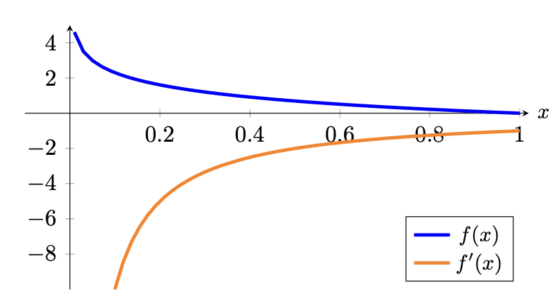
Categorical cross-entropy loss function (blue) and gradient (orange)

Notice that the loss is exactly 0 if the probability of the ground truth class is 1 as desired. Also, as the probability of the ground truth class tends to 0, the loss tends to positive infinity as well, hence substantially penalizing bad predictions. You might recognize this loss function for logistic regression, which is similar except the logistic regression loss is specific to the case of binary classes.

Looking at the gradient, you can see that the gradient is generally negative, which is also expected since, to decrease this loss, you would want the probability on the ground truth class to be as high as possible. Recall that gradient descent goes in the opposite direction of the gradient.

In PyTorch, the cross-entropy function is provided by nn.CrossEntropyLoss(). It takes the predicted logits and the target as parameter and compute the categorical cross-entropy. Remind that inside the CrossEntropyLoss() function, softmax will be applied to the logits hence you should not use softmax activation function at the output layer. Example of using the cross entropy loss function from PyTorch is as follows:

It prints:

Note the first argument to the cross entropy loss function is logit, not probabilities. Hence each row does not sum to 1. The second argument, however, is a tensor containing rows of probabilities. If you convert the logits tensor above into probability using softmax function, it would be:

which each row sums to 1.0. This tensor also reveals why the cross entropy above calculated to be 0.288, which is $-\log(0.75)$.

The other way of calculating the cross entropy in PyTorch is not to use one-hot encoding in the target but to use the integer indices label:

This gives you the same cross entropy of 0.288. Note that,

gives you:

This is how PyTorch interprets your target tensor. It is also called “sparse cross entropy” function in other libraries, to make a distinction that it does not expect a one-hot vector.

Note in PyTorch, you can use nn.LogSoftmax() as an activation function. It is to apply softmax on the output of a layer and than take the logarithm on each element. If this is your output layer, you should use nn.NLLLoss() (negative log likelihood) as the loss function. Mathematically these duo is same as cross entropy loss. You can confirm this by checking the code below produced the same output:

In case of a classification problem with only two classes, it becomes binary classification. It is special because the model is now a logistic regression model in which there can be only one output instead of a vector of two values. You can still implement binary classification as multiclass classification and use the same cross entropy function. But if you output $x$ as the probability (between 0 and 1) for the “positive class”, it is known that the probability for the “negative class” must be $1-x$.

In PyTorch, you have nn.BCELoss() for binary cross entropy. It is specialized for binary case. For example:

This gives you:

It is because:

$$\frac{1}{2}[-\log(0.75) + (-\log(1-0.25))] = -\log(0.75) = 0.288$$

Note that in PyTorch, the target label 1 is taken as the “positive class” and label 0 is the “negative class”. There should not be other values in the target tensor.

Custom Loss Function in PyTorch

Notice in above, the loss metric is calculated using an object from torch.nn module. The loss metric computed is a PyTorch tensor, so you can differentiate it and start the backpropagation. Therefore, nothing forbid you from creating your own loss function as long as you can compute a tensor based on the model’s output.

PyTorch does not give you all the possible loss metrics. For example, mean absolute percentage error is not included. It is like MAE, defined as:

$$\text{MAPE} = \frac{1}{m} \sum_{i=1}^m \lvert\frac{\hat{y}_i – y_i}{y_i}\rvert$$

Sometimes you may prefer to use MAPE. Recall the example on regression on the California housing dataset, the prediction is on the house price. It may make more sense to consider prediction accurate based on percentage difference rather than dollar difference. You can define your MAPE function, just remember to use PyTorch functions to compute, and return a PyTorch tensor.

See the full example below:

Compare to the example in the other post, you can see that loss_fn now is defined as a custom function. Otherwise everything is just the same.

Further Readings

Below are the documentations from PyTorch that give you more details on how the various loss functions are implemented:

• nn.L1Loss from PyTorch
• nn.MSELoss from PyTorch
• nn.CrossEntropyLoss from PyTorch
• nn.BCELoss from PyTorch
• nn.NLLLoss from PyTorch

Summary

In this post, you have seen loss functions and the role that they play in a neural network. You have also seen some popular loss functions used in regression and classification models, as well as how to implement your own loss function for your PyTorch model. Specifically, you learned:

• What are loss functions, and why they are important in training
• Common loss functions for regression and classification problems
• How to use loss functions in your PyTorch model

Get Started on Deep Learning with PyTorch!

Learn how to build deep learning models

...using the newly released PyTorch 2.0 library

Discover how in my new Ebook:
Deep Learning with PyTorch

It provides self-study tutorials with hundreds of working code to turn you from a novice to expert. It equips you with
tensor operation, training, evaluation, hyperparameter optimization, and much more...

Kick-start your deep learning journey with hands-on exercises

See What's Inside