Data transformations enable data scientists to refine, normalize, and standardize raw data into a format ripe for analysis. These transformations are not merely procedural steps; they are essential in mitigating biases, handling skewed distributions, and enhancing the robustness of statistical models. This chapter will primarily focus on how to address skewed data. By focusing on the “SalePrice” and “YearBuilt” attributes from the Ames housing dataset, you will see examples of positive and negative skewed data and ways to normalize their distributions using transformations.
Let’s get started.

Skewness Be Gone: Transformative Tricks for Data Scientists
Photo by Suzanne D. Williams. Some rights reserved.
Overview
This post is divided into five parts; they are:
- Understanding Skewness and the Need for Transformation
- Strategies for Taming Positive Skewness
- Strategies for Taming Negative Skewness
- Statistical Evaluation of Transformations
- Choosing the Right Transformation
Understanding Skewness and the Need for Transformation
Skewness is a statistical measure that describes the asymmetry of a data distribution around its mean. In simpler terms, it indicates whether the bulk of the data is bunched up on one side of the scale, leaving a long tail stretching out in the opposite direction. There are two types of skewness you encounter in data analysis:
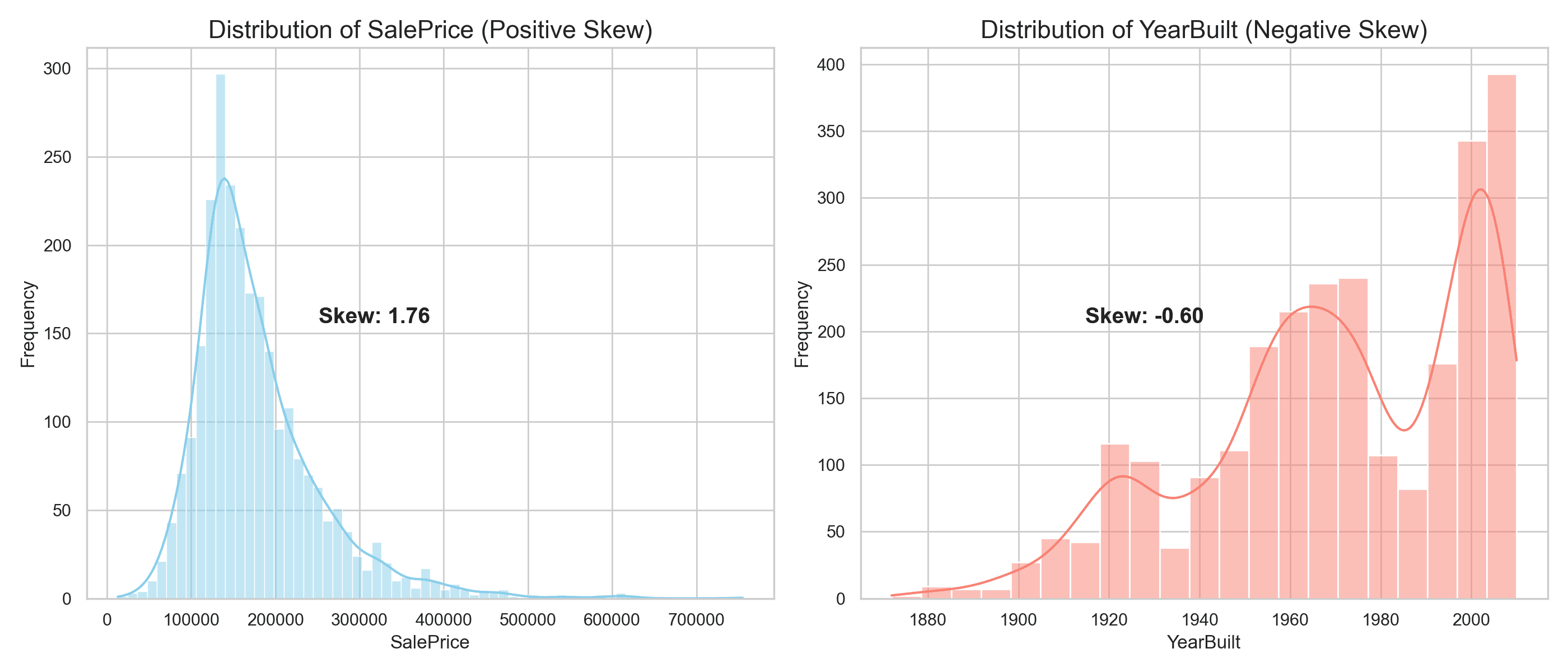
- Positive Skewness: This occurs when the tail of the distribution extends towards higher values, on the right side of the peak. The majority of data points are clustered at the lower end of the scale, indicating that while most values are relatively low, there are a few exceptionally high values. The ‘SalePrice’ attribute in the Ames dataset exemplifies positive skewness, as most homes sell at lower prices, but a small number sell at significantly higher prices.
- Negative Skewness: Conversely, negative skewness happens when the tail of the distribution stretches towards lower values, on the left side of the peak. In this scenario, the data is concentrated towards the higher end of the scale, with fewer values trailing off into lower numbers. The ‘YearBuilt’ feature of the Ames dataset is a perfect illustration of negative skewness, suggesting that while a majority of houses were built in more recent years, a smaller portion dates back to earlier times.
To better grasp these concepts, let’s visualize the skewness.
|
1 2 3 4 5 6 7 8 9 10 11 12 13 14 15 16 17 18 19 20 21 22 23 24 25 26 27 28 29 30 31 32 33 34 35 36 37 38 39 40 41 42 43 |
# Import the necessary libraries import pandas as pd import matplotlib.pyplot as plt import seaborn as sns import numpy as np from scipy.stats import boxcox, yeojohnson from sklearn.preprocessing import QuantileTransformer # Load the dataset Ames = pd.read_csv('Ames.csv') # Calculate skewness sale_price_skew = Ames['SalePrice'].skew() year_built_skew = Ames['YearBuilt'].skew() # Set the style of seaborn sns.set(style='whitegrid') # Create a figure for 2 subplots (1 row, 2 columns) fig, ax = plt.subplots(1, 2, figsize=(14, 6)) # Plot for SalePrice (positively skewed) sns.histplot(Ames['SalePrice'], kde=True, ax=ax[0], color='skyblue') ax[0].set_title('Distribution of SalePrice (Positive Skew)', fontsize=16) ax[0].set_xlabel('SalePrice') ax[0].set_ylabel('Frequency') # Annotate Skewness ax[0].text(0.5, 0.5, f'Skew: {sale_price_skew:.2f}', transform=ax[0].transAxes, horizontalalignment='right', color='black', weight='bold', fontsize=14) # Plot for YearBuilt (negatively skewed) sns.histplot(Ames['YearBuilt'], kde=True, ax=ax[1], color='salmon') ax[1].set_title('Distribution of YearBuilt (Negative Skew)', fontsize=16) ax[1].set_xlabel('YearBuilt') ax[1].set_ylabel('Frequency') # Annotate Skewness ax[1].text(0.5, 0.5, f'Skew: {year_built_skew:.2f}', transform=ax[1].transAxes, horizontalalignment='right', color='black', weight='bold', fontsize=14) plt.tight_layout() plt.show() |
For ‘SalePrice’, the graph shows a pronounced right-skewed distribution, highlighting the challenge of skewness in data analysis. Such distributions can complicate predictive modeling and obscure insights, making it difficult to draw accurate conclusions. In contrast, ‘YearBuilt’ demonstrates negative skewness, where the distribution reveals that newer homes predominate, with older homes forming the long tail to the left.
Addressing skewness through data transformation is not merely a statistical adjustment; it is a crucial step toward uncovering precise, actionable insights. By applying transformations, you aim to mitigate the effects of skewness, facilitating more reliable and interpretable analyses. This normalization process enhances your ability to conduct meaningful data science, beyond just meeting statistical prerequisites. It underscores your commitment to improving the clarity and utility of your data, setting the stage for insightful, impactful findings in your subsequent explorations of data transformation.
Kick-start your project with my book The Beginner’s Guide to Data Science. It provides self-study tutorials with working code.
Strategies for Taming Positive Skewness
To combat positive skew, you can use five key transformations: Log, Square Root, Box-Cox, Yeo-Johnson, and Quantile Transformations. Each method aims to mitigate skewness, enhancing the data’s suitability for further analysis.
Log Transformation
This method is particularly suited for right-skewed data, effectively minimizing large-scale differences by taking the natural log of all data points. This compression of the data range makes it more amenable for further statistical analysis.
|
1 2 3 |
# Applying Log Transformation Ames['Log_SalePrice'] = np.log(Ames['SalePrice']) print(f"Skewness after Log Transformation: {Ames['Log_SalePrice'].skew():.5f}") |
You can see that the skewness is reduced:
|
1 |
Skewness after Log Transformation: 0.04172 |
Square Root Transformation
A softer approach than the log transformation, ideal for moderately skewed data. By applying the square root to each data point, it reduces skewness and diminishes the impact of outliers, making the distribution more symmetric.
|
1 2 3 |
# Applying Square Root Transformation Ames['Sqrt_SalePrice'] = np.sqrt(Ames['SalePrice']) print(f"Skewness after Square Root Transformation: {Ames['Sqrt_SalePrice'].skew():.5f}") |
This prints:
|
1 |
Skewness after Square Root Transformation: 0.90148 |
Box-Cox Transformation
Offers flexibility by optimizing the transformation parameter lambda (λ), applicable only to positive data. The Box-Cox method systematically finds the best power transformation to reduce skewness and stabilize variance, enhancing the data’s normality.
|
1 2 3 4 5 6 7 |
# Applying Box-Cox Transformation after checking all values are positive if (Ames['SalePrice'] > 0).all(): Ames['BoxCox_SalePrice'], _ = boxcox(Ames['SalePrice']) else: # Consider alternative transformations or handling strategies print("Not all SalePrice values are positive. Consider using Yeo-Johnson or handling negative values.") print(f"Skewness after Box-Cox Transformation: {Ames['BoxCox_SalePrice'].skew():.5f}") |
This is the best transformation so far because the skewness is very close to zero:
|
1 |
Skewness after Box-Cox Transformation: -0.00436 |
Yeo-Johnson Transformation
The above transformations only work with positive data. Yeo-Johnson is similar to Box-Cox but adaptable to both positive and non-positive data. It modifies the data through an optimal transformation parameter. This adaptability allows it to manage skewness across a wider range of data values, improving its fit for statistical models.
|
1 2 3 |
# Applying Yeo-Johnson Transformation Ames['YeoJohnson_SalePrice'], _ = yeojohnson(Ames['SalePrice']) print(f"Skewness after Yeo-Johnson Transformation: {Ames['YeoJohnson_SalePrice'].skew():.5f}") |
Similar to Box-Cox, the skewness after transformation is very close to zero:
|
1 |
Skewness after Yeo-Johnson Transformation: -0.00437 |
Quantile Transformation
Quantile transformation maps data to a specified distribution, such as normal, effectively addresses skewness by distributing the data points evenly across the chosen distribution. This transformation normalizes the shape of the data, focusing on making the distribution more uniform or Gaussian-like without assuming it will directly benefit linear models due to its non-linear nature and the challenge of reverting the data to its original form.
|
1 2 3 4 |
# Applying Quantile Transformation to follow a normal distribution quantile_transformer = QuantileTransformer(output_distribution='normal', random_state=0) Ames['Quantile_SalePrice'] = quantile_transformer.fit_transform(Ames['SalePrice'].values.reshape(-1, 1)).flatten() print(f"Skewness after Quantile Transformation: {Ames['Quantile_SalePrice'].skew():.5f}") |
Because this transformation fits the data into the Gaussian distribution by brute force, the skewness is closest to zero:
|
1 |
Skewness after Quantile Transformation: 0.00286 |
To illustrate the effects of these transformations, let’s take a look at the visual representation of the ‘SalePrice’ distribution before and after each method is applied.
|
1 2 3 4 5 6 7 8 9 10 11 12 13 14 15 16 17 18 19 20 21 22 23 24 25 26 27 28 29 30 31 32 33 34 35 36 37 38 39 40 41 42 43 44 45 46 47 48 |
# Plotting the distributions fig, axes = plt.subplots(2, 3, figsize=(18, 15)) # Adjusted for an additional plot # Flatten the axes array for easier indexing axes = axes.flatten() # Hide unused subplot axes for ax in axes[6:]: ax.axis('off') # Original SalePrice Distribution sns.histplot(Ames['SalePrice'], kde=True, bins=30, color='skyblue', ax=axes[0]) axes[0].set_title('Original SalePrice Distribution (Skew: 1.76)') axes[0].set_xlabel('SalePrice') axes[0].set_ylabel('Frequency') # Log Transformed SalePrice sns.histplot(Ames['Log_SalePrice'], kde=True, bins=30, color='blue', ax=axes[1]) axes[1].set_title('Log Transformed SalePrice (Skew: 0.04172)') axes[1].set_xlabel('Log of SalePrice') axes[1].set_ylabel('Frequency') # Square Root Transformed SalePrice sns.histplot(Ames['Sqrt_SalePrice'], kde=True, bins=30, color='orange', ax=axes[2]) axes[2].set_title('Square Root Transformed SalePrice (Skew: 0.90148)') axes[2].set_xlabel('Square Root of SalePrice') axes[2].set_ylabel('Frequency') # Box-Cox Transformed SalePrice sns.histplot(Ames['BoxCox_SalePrice'], kde=True, bins=30, color='red', ax=axes[3]) axes[3].set_title('Box-Cox Transformed SalePrice (Skew: -0.00436)') axes[3].set_xlabel('Box-Cox of SalePrice') axes[3].set_ylabel('Frequency') # Yeo-Johnson Transformed SalePrice sns.histplot(Ames['YeoJohnson_SalePrice'], kde=True, bins=30, color='purple', ax=axes[4]) axes[4].set_title('Yeo-Johnson Transformed SalePrice (Skew: -0.00437)') axes[4].set_xlabel('Yeo-Johnson of SalePrice') axes[4].set_ylabel('Frequency') # Quantile Transformed SalePrice (Normal Distribution) sns.histplot(Ames['Quantile_SalePrice'], kde=True, bins=30, color='green', ax=axes[5]) axes[5].set_title('Quantile Transformed SalePrice (Normal Distn, Skew: 0.00286)') axes[5].set_xlabel('Quantile Transformed SalePrice') axes[5].set_ylabel('Frequency') plt.tight_layout(pad=4.0) plt.show() |
The following visual provides a side-by-side comparison, helping you to understand better the influence of each transformation on the distribution of housing prices.
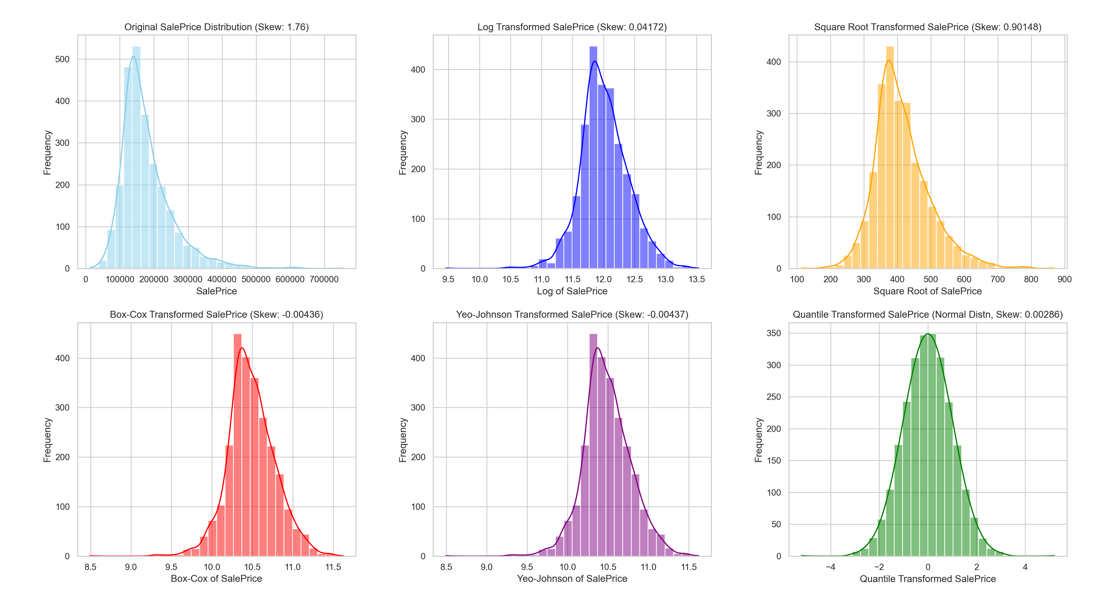
Distribution of data after transformation
This visual serves as a clear reference for how each transformation method alters the distribution of ‘SalePrice’, demonstrating the resulting effect towards achieving a more normal distribution.
Strategies for Taming Negative Skewness
To combat negative skew, you can use the five key transformations: Squared, Cubed, Box-Cox, Yeo-Johnson, and Quantile Transformations. Each method aims to mitigate skewness, enhancing the data’s suitability for further analysis.
Squared Transformation
This involves taking each data point in the dataset and squaring it (i.e., raising it to the power of 2). The squared transformation is useful for reducing negative skewness because it tends to spread out the lower values more than the higher values. However, it’s more effective when all data points are positive and the degree of negative skewness is not extreme.
|
1 2 3 |
# Applying Squared Transformation Ames['Squared_YearBuilt'] = Ames['YearBuilt'] ** 2 print(f"Skewness after Squared Transformation: {Ames['Squared_YearBuilt'].skew():.5f}") |
It prints:
|
1 |
Skewness after Squared Transformation: -0.57207 |
Cubed Transformation
Similar to the squared transformation but involves raising each data point to the power of 3. The cubed transformation can further reduce negative skewness, especially in cases where the squared transformation is insufficient. It’s more aggressive in spreading out values, which can benefit more negatively skewed distributions.
|
1 2 3 |
# Applying Cubed Transformation Ames['Cubed_YearBuilt'] = Ames['YearBuilt'] ** 3 print(f"Skewness after Cubed Transformation: {Ames['Cubed_YearBuilt'].skew():.5f}") |
It prints:
|
1 |
Skewness after Cubed Transformation: -0.54539 |
Box-Cox Transformation
A more sophisticated method that finds the best lambda (λ) parameter to transform the data into a normal shape. The transformation is defined for positive data only. The Box-Cox transformation is highly effective for a wide range of distributions, including those with negative skewness, by making the data more symmetric. For negatively skewed data, a positive lambda is often found, applying a transformation that effectively reduces skewness.
|
1 2 3 4 5 6 7 |
# Applying Box-Cox Transformation after checking all values are positive if (Ames['YearBuilt'] > 0).all(): Ames['BoxCox_YearBuilt'], _ = boxcox(Ames['YearBuilt']) else: # Consider alternative transformations or handling strategies print("Not all YearBuilt values are positive. Consider using Yeo-Johnson or handling negative values.") print(f"Skewness after Box-Cox Transformation: {Ames['BoxCox_YearBuilt'].skew():.5f}") |
You can see the skewness is moved closer to zero than before:
|
1 |
Skewness after Box-Cox Transformation: -0.12435 |
Yeo-Johnson Transformation
Similar to the Box-Cox transformation, but the Yeo-Johnson is designed to handle both positive and negative data. For negatively skewed data, the Yeo-Johnson transformation can normalize distributions even when negative values are present. It adjusts the data in a way that reduces skewness, making it particularly versatile for datasets with a mix of positive and negative values.
|
1 2 3 |
# Applying Yeo-Johnson Transformation Ames['YeoJohnson_YearBuilt'], _ = yeojohnson(Ames['YearBuilt']) print(f"Skewness after Yeo-Johnson Transformation: {Ames['YeoJohnson_YearBuilt'].skew():.5f}") |
Similar to Box-Cox, you get a skewness moved closer to zero:
|
1 |
Skewness after Yeo-Johnson Transformation: -0.12435 |
Quantile Transformation
This method transforms the features to follow a specified distribution, such as the normal distribution, based on their quantiles. It does not assume any specific distribution shape for the input data. When applied to negatively skewed data, the quantile transformation can effectively normalize the distribution. It’s particularly useful for dealing with outliers and making the distribution of the data uniform or normal, regardless of the original skewness.
|
1 2 3 4 |
# Applying Quantile Transformation to follow a normal distribution quantile_transformer = QuantileTransformer(output_distribution='normal', random_state=0) Ames['Quantile_YearBuilt'] = quantile_transformer.fit_transform(Ames['YearBuilt'].values.reshape(-1, 1)).flatten() print(f"Skewness after Quantile Transformation: {Ames['Quantile_YearBuilt'].skew():.5f}") |
As you saw before in the case of positive skewness, quantile transformation provides the best result in the sense that the resulting skewness is closest to zero:
|
1 |
Skewness after Quantile Transformation: 0.02713 |
To illustrate the effects of these transformations, let’s take a look at the visual representation of the ‘YearBuilt’ distribution before and after each method is applied.
|
1 2 3 4 5 6 7 8 9 10 11 12 13 14 15 16 17 18 19 20 21 22 23 24 25 26 27 28 29 30 31 32 33 34 35 36 37 38 39 40 41 42 43 44 |
# Plotting the distributions fig, axes = plt.subplots(2, 3, figsize=(18, 15)) # Flatten the axes array for easier indexing axes = axes.flatten() # Original YearBuilt Distribution sns.histplot(Ames['YearBuilt'], kde=True, bins=30, color='skyblue', ax=axes[0]) axes[0].set_title(f'Original YearBuilt Distribution (Skew: {Ames["YearBuilt"].skew():.5f})') axes[0].set_xlabel('YearBuilt') axes[0].set_ylabel('Frequency') # Squared YearBuilt sns.histplot(Ames['Squared_YearBuilt'], kde=True, bins=30, color='blue', ax=axes[1]) axes[1].set_title(f'Squared YearBuilt (Skew: {Ames["Squared_YearBuilt"].skew():.5f})') axes[1].set_xlabel('Squared YearBuilt') axes[1].set_ylabel('Frequency') # Cubed YearBuilt sns.histplot(Ames['Cubed_YearBuilt'], kde=True, bins=30, color='orange', ax=axes[2]) axes[2].set_title(f'Cubed YearBuilt (Skew: {Ames["Cubed_YearBuilt"].skew():.5f})') axes[2].set_xlabel('Cubed YearBuilt') axes[2].set_ylabel('Frequency') # Box-Cox Transformed YearBuilt sns.histplot(Ames['BoxCox_YearBuilt'], kde=True, bins=30, color='red', ax=axes[3]) axes[3].set_title(f'Box-Cox Transformed YearBuilt (Skew: {Ames["BoxCox_YearBuilt"].skew():.5f})') axes[3].set_xlabel('Box-Cox YearBuilt') axes[3].set_ylabel('Frequency') # Yeo-Johnson Transformed YearBuilt sns.histplot(Ames['YeoJohnson_YearBuilt'], kde=True, bins=30, color='purple', ax=axes[4]) axes[4].set_title(f'Yeo-Johnson Transformed YearBuilt (Skew: {Ames["YeoJohnson_YearBuilt"].skew():.5f})') axes[4].set_xlabel('Yeo-Johnson YearBuilt') axes[4].set_ylabel('Frequency') # Quantile Transformed YearBuilt (Normal Distribution) sns.histplot(Ames['Quantile_YearBuilt'], kde=True, bins=30, color='green', ax=axes[5]) axes[5].set_title(f'Quantile Transformed YearBuilt (Normal Distn, Skew: {Ames["Quantile_YearBuilt"].skew():.5f})') axes[5].set_xlabel('Quantile Transformed YearBuilt') axes[5].set_ylabel('Frequency') plt.tight_layout(pad=4.0) plt.show() |
The following visual provides a side-by-side comparison, helping us to better understand the influence of each transformation on this feature.
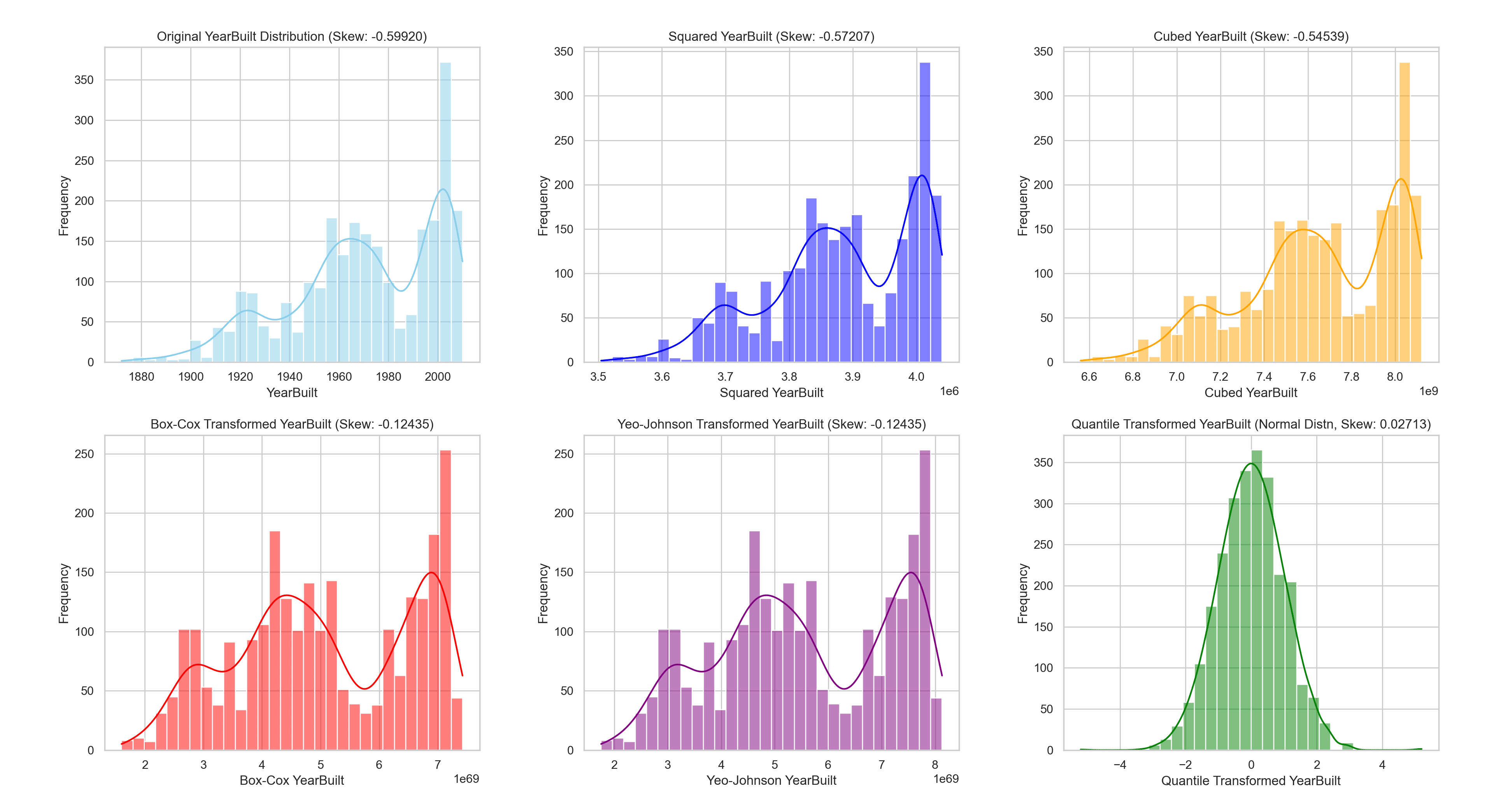
This visual provides a clear reference for how each transformation method alters the distribution of ‘YearBuilt’, demonstrating the resulting effect towards achieving a more normal distribution.
Want to Get Started With Beginner's Guide to Data Science?
Take my free email crash course now (with sample code).
Click to sign-up and also get a free PDF Ebook version of the course.
Statistical Evaluation of Transformations
How do you know the transformed data matches the normal distribution?
The Kolmogorov-Smirnov (KS) test is a non-parametric test used to determine if a sample comes from a population with a specific distribution. Unlike parametric tests, which assume a specific distribution form for the data (usually normal distribution), non-parametric tests make no such assumptions. This quality makes them highly useful in the context of data transformations because it helps to assess how closely a transformed dataset approximates a normal distribution. The KS test compares the cumulative distribution function (CDF) of the sample data against the CDF of a known distribution (in this case, the normal distribution), providing a test statistic that quantifies the distance between the two.
Null and Alternate Hypothesis:
- Null Hypothesis ($H_0$): The data follows the specified distribution (normal distribution, in this case).
- Alternate Hypothesis ($H_1$): The data does not follow the specified distribution.
In this context, the KS test is used to evaluate the goodness-of-fit between the empirical distribution of the transformed data and the normal distribution. The test statistic is a measure of the largest discrepancy between the empirical (transformed data) and theoretical CDFs (normal distribution). A small test statistic suggests that the distributions are similar.
|
1 2 3 4 5 6 7 8 9 10 11 12 13 14 15 16 17 18 19 |
# Import the Kolmogorov-Smirnov Test from scipy.stats from scipy.stats import kstest # Run the KS tests for the 10 cases transformations = ["Log_SalePrice", "Sqrt_SalePrice", "BoxCox_SalePrice", "YeoJohnson_SalePrice", "Quantile_SalePrice", "Squared_YearBuilt", "Cubed_YearBuilt", "BoxCox_YearBuilt", "YeoJohnson_YearBuilt", "Quantile_YearBuilt"] # Standardizing the transformations before performing KS test ks_test_results = {} for transformation in transformations: standardized_data = (Ames[transformation] - Ames[transformation].mean()) / Ames[transformation].std() ks_stat, ks_p_value = kstest(standardized_data, 'norm') ks_test_results[transformation] = (ks_stat, ks_p_value) # Convert results to DataFrame for easier comparison ks_test_results_df = pd.DataFrame.from_dict(ks_test_results, orient='index', columns=['KS Statistic', 'P-Value']) print(ks_test_results_df.round(5)) |
The code above prints a table as follows:
|
1 2 3 4 5 6 7 8 9 10 11 |
KS Statistic P-Value Log_SalePrice 0.04261 0.00017 Sqrt_SalePrice 0.07689 0.00000 BoxCox_SalePrice 0.04294 0.00014 YeoJohnson_SalePrice 0.04294 0.00014 Quantile_SalePrice 0.00719 0.99924 Squared_YearBuilt 0.11661 0.00000 Cubed_YearBuilt 0.11666 0.00000 BoxCox_YearBuilt 0.11144 0.00000 YeoJohnson_YearBuilt 0.11144 0.00000 Quantile_YearBuilt 0.02243 0.14717 |
You can see that the higher the KS statistic, the lower the p-value. Respectively,
- KS Statistic: This represents the maximum difference between the empirical distribution function of the sample and the cumulative distribution function of the reference distribution. Smaller values indicate a closer fit to the normal distribution.
- P-Value: Provides the probability of observing the test results under the null hypothesis. A low p-value (typically <0.05) rejects the null hypothesis, indicating the sample distribution significantly differs from the normal distribution.
The Quantile transformation of ‘SalePrice’ yielded the most promising results, with a KS statistic of 0.00719 and a p-value of 0.99924, indicating that after this transformation, the distribution closely aligns with the normal distribution. It is not surprising because Quantile Transformation is designed to produce a good fit. The p-value is significant because a higher p-value (close to 1) suggests that the null hypothesis (that the sample comes from a specified distribution) cannot be rejected, implying good normality.
Other transformations like Log, Box-Cox, and Yeo-Johnson also improved the distribution of ‘SalePrice’ but to a lesser extent, as reflected by their lower p-values (ranging from 0.00014 to 0.00017), indicating less conformity to the normal distribution compared to the Quantile transformation. The transformations applied to ‘YearBuilt’ showed generally less effectiveness in achieving normality compared to ‘SalePrice’. The BoxCox and YeoJohnson transformations offered slight improvements over Squaring and Cubing, as seen in their slightly lower KS statistics and p-values, but still indicated significant deviations from normality. The Quantile transformation for ‘YearBuilt’ showed a more favorable outcome with a KS statistic of 0.02243 and a p-value of 0.14717, suggesting a moderate improvement towards normality, although not as pronounced as the effect seen with ‘SalePrice’.
Choosing the Right Transformation
Choosing the right transformation for addressing skewness in data is not a one-size-fits-all decision; it requires careful consideration of the context and characteristics of the data at hand. The importance of context in selecting the appropriate transformation method cannot be overstated. Here are key factors to consider:
- Data Characteristics: The nature of the data (e.g., the presence of zeros or negative values) can limit the applicability of certain transformations. For instance, log transformations cannot be directly applied to zero or negative values without adjustments.
- Degree of Skewness: The extent of skewness in the data influences the choice of transformation. More severe skewness might require more potent transformations (e.g., Box-Cox or Yeo-Johnson) compared to milder skewness, which might be adequately addressed with log or square root transformations.
- Statistical Properties: The transformation chosen should ideally improve the statistical properties of the dataset, such as normalizing the distribution and stabilizing variance, which are essential for many statistical tests and models.
- Interpretability: The ease of interpreting results after transformation is crucial. Some transformations, like log or square root, allow for relatively straightforward interpretation, whereas others, like the quantile transformation, might complicate the original scale’s interpretation.
- Objective of Analysis: The ultimate goal of the analysis—whether it’s predictive modeling, hypothesis testing, or exploratory analysis—plays a critical role in selecting the transformation method. The transformation should align with the analytical techniques and models to be employed later.
In summary, the choice of the right transformation depends on multiple factors, including, but not limited to, a solid understanding of the dataset, the specific goals of the analysis, and the practical implications for model interpretability and performance. No single method is universally superior; each has its trade-offs and applicability depending on the scenario at hand. It’s important to highlight a cautionary note regarding the Quantile Transformation, which your visual and statistical tests identified as highly effective in achieving a normal distribution. While potent, the Quantile Transformation is not a linear transformation like the others. This means it can significantly alter the data’s structure in ways that are not easily reversible, potentially complicating the interpretation of results and the application of inverse transformations for back-transformation to the original scale. Therefore, despite its effectiveness in normalization, its use should be considered carefully, especially in cases where maintaining a connection to the original data scale is important or where the model’s interpretability is a priority. In most scenarios, the preference might lean towards transformations that balance normalization effectiveness with simplicity and reversibility, ensuring that the data remains as interpretable and manageable as possible.
Further Reading
APIs
- scipy.stats.boxcox API
- scipy.stats.yeojohnson API
- sklearn.preprocessing.Quantile Transformer API
- scipy.stats.kstest API
Resources
Summary
In this post, you’ve embarked on a detailed exploration of data transformations, focusing on their critical role in addressing skewed data within the field of data science. Through practical examples using the ‘SalePrice’ and ‘YearBuilt’ features from the Ames housing dataset, you demonstrated various transformation techniques—log, square root, Box-Cox, Yeo-Johnson, and quantile transformations—and their impact on normalizing data distributions. Your analysis underscores the necessity of selecting appropriate transformations based on data characteristics, the degree of skewness, statistical goals, interpretability, and the specific objectives of the analysis.
Specifically, you learned:
- The significance of data transformations and how they can handle skewed distributions.
- How to compare the effectiveness of different transformations through visual and statistical assessments.
- The importance of evaluating data characteristics, the severity of skewness, and analytical objectives to choose the most suitable transformation technique.
Do you have any questions? Please ask your questions in the comments below, and I will do my best to answer.
Get Started on The Beginner's Guide to Data Science!
Learn the mindset to become successful in data science projects
...using only minimal math and statistics, acquire your skill through short examples in Python
Discover how in my new Ebook:
The Beginner's Guide to Data Science
It provides self-study tutorials with all working code in Python to turn you from a novice to an expert. It shows you how to find outliers, confirm the normality of data, find correlated features, handle skewness, check hypotheses, and much more...all to support you in creating a narrative from a dataset.


")


No comments yet.