How to Build a Robust RAG System with Minimal Resources

In this article, you will learn how to design, assemble, and tune a retrieval-augmented generation system that runs entirely on a standard laptop, without cloud infrastructure or paid APIs.

Topics we will cover include:

• How quantization, compact embedding models, and in-process vector stores make a full RAG pipeline possible on consumer hardware.
• Which lightweight packages handle each stage of the pipeline, from document ingestion and chunking through retrieval, prompting, and local generation.
• How to make the system reliable through source citations, retrieval thresholds, evaluation sets, and query logs that distinguish retrieval failures from generation failures.

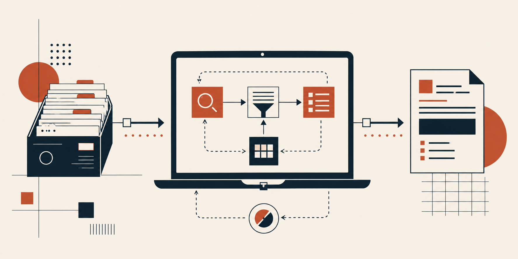
Introduction

Retrieval-augmented generation, or RAG, connects a language model to your own collection of documents so it answers from your material instead of guessing. Most build guides assume a cloud GPU, a hosted vector database, and a paid API that charges you for every question. None of that is required. A laptop with 8 GB or 16 GB of RAM can run a complete RAG system that stays offline, costs nothing per query, and keeps sensitive documents on your own machine.

This guide covers the architecture and the package choices that make a small setup hold up rather than fall over. There’s no code here on purpose. A working RAG system spans document loading, chunking, embedding, storage, retrieval, prompting, and generation, and no short snippet represents that honestly. Each section explains what a component does, which lightweight package handles it, and where to find a tested implementation you can copy and adapt.

Defining What “Minimal Resources” Means Here

Minimal means no dedicated GPU, no monthly bill, and no data leaving your machine. Three choices make that possible.

The first is quantization. Model weights are normally stored at 16 bits per parameter, and quantized formats such as GGUF compress them to 4 or 5 bits. That cuts memory use by roughly two thirds at a small accuracy cost. A 7 billion parameter model that needs 14 GB at full precision runs in about 4 GB once quantized.

The second is a small embedding model. Embeddings turn text into numeric vectors so similar passages sit close together. Compact sentence encoders around 80 MB in size produce 384-dimensional vectors and handle retrieval well for most document collections.

The third is a local vector store that runs inside your Python process instead of as a separate database server.

Set your speed expectations accordingly. On CPU-only hardware, generation runs at a few tokens per second. That suits a research assistant or an internal knowledge tool, not a high-traffic public application.

Assembling the Small-Footprint Toolkit

These are the packages worth knowing before you start.

• Orchestration: LangChain connects the pieces and supplies document loaders, text splitters, and retriever interfaces. LlamaIndex is a reasonable alternative with a stronger focus on indexing.
• Local inference: llama.cpp is a C and C++ implementation of language model inference tuned for CPUs, exposed to Python through the llama-cpp-python package. Ollama wraps similar functionality behind a simpler command line and local server.
• Embeddings: sentence-transformers from Hugging Face downloads and runs compact encoder models locally, with no API calls.
• Vector storage: FAISS gives you fast similarity search over an in-memory index that you save to disk. ChromaDB adds metadata filtering and persistence, with a bit more setup.
• Document parsing: pypdf handles PDFs. The unstructured package covers a wider mix of file formats.
• Interface: Streamlit turns your pipeline into a browser-based tool in a few dozen lines.

For a complete offline build using llama.cpp, LangChain, and ChromaDB together, follow Building a RAG Pipeline with llama.cpp in Python. For the FAISS and Hugging Face variant, see A Practical Guide to Building Local RAG Applications with LangChain.

Step 1: Ingesting and Chunking Your Documents

Your system is only as good as the text you feed it. Load each document, strip page headers and footers, then split the text into chunks.

Chunk size drives retrieval quality more than almost anything else. Chunks of 500 to 1000 characters with 10 to 20 percent overlap are a good starting point. Too small, and a chunk loses the context needed to answer anything. Too large, and the retrieved passage buries the relevant sentence in noise, wasting space in a small model’s limited context window.

Split on natural boundaries where you can. Paragraph breaks and section headings preserve meaning better than a fixed character count. Attach metadata to every chunk as you create it: source filename, page number, and section title. That metadata lets you filter searches and cite sources in your answers later.

For a walkthrough of chunking dense academic PDFs, including a Streamlit interface, see Let’s Build a RAG-Powered Research Paper Assistant.

Step 2: Embedding and Indexing Your Chunks

Each chunk goes through the embedding model once and comes back as a vector. Those vectors go into your index alongside the original text and metadata.

Two rules keep this stage from causing trouble later. Use the same embedding model for indexing and querying, since vectors from different models are not comparable. And save the index to disk, because re-embedding thousands of chunks on CPU takes minutes you don’t need to spend twice.

A few thousand documents produce an index measured in tens of megabytes, which FAISS searches in milliseconds. Rebuild only when documents change or when you switch embedding models.

Step 3: Retrieving and Prompting

At query time, the user’s question is embedded with the same model, and the index returns the closest chunks. Four to six chunks suits a small model with a modest context window.

Plain similarity search misses more often than people expect. Short questions produce vague vectors, and phrasing that differs from the source text drops the match score. Two techniques address this cheaply. Query expansion rewrites the question into several variants and pools the results. Hypothetical document embeddings, or HyDE, ask the model to draft a plausible answer first, then search using that draft. An invented answer resembles the target passage more closely than a question does.

The prompt you build around the retrieved text matters just as much. Tell the model to answer only from the supplied context, and to say it doesn’t know when the context falls short. Prompt Engineering Patterns for Successful RAG Implementations covers these retrieval prompting patterns in detail.

Step 4: Generating Answers Locally

The retrieved chunks and your instructions go to the local model. A quantized 7B or 8B instruction-tuned model handles grounded question answering well. Smaller 3B models respond faster and suit narrow tasks.

Two settings deserve attention. Set the context length high enough to hold your retrieved chunks plus the question plus the answer. And keep temperature low, around 0.1 to 0.3, since factual answers drawn from source documents shouldn’t be creative.

Making the System Reliable

Reliability comes from grounding, and from knowing when the system has failed.

Require citations. When every claim carries a source filename and page number, wrong answers become visible instead of hiding behind confident phrasing.

Set a similarity threshold. If the best retrieved chunk scores below your cutoff, return a message saying the answer isn’t in the knowledge base rather than passing weak context to the model.

Build a small evaluation set. Twenty to thirty questions with known correct answers, rechecked after each change to chunk size or embedding model, tell you whether an adjustment helped. Without this, tuning is guesswork.

Log the retrieved chunks for every query. When an answer is wrong, the log shows straight away whether retrieval failed or generation failed, and those two problems have completely different fixes.

Knowing When to Scale Up

A small local system covers a lot of ground, but some problems need more.

Questions that connect facts across several documents expose the limits of similarity search. Graph-based retrieval, which stores entities and relationships rather than isolated chunks, handles that pattern better. See Building a Graph RAG System: A Step-by-Step Approach.

Specialized domains sometimes need a generator model trained to interpret retrieved passages more reliably, covered in Understanding RAG Part IX: Fine-Tuning LLMs for RAG. And when a prototype becomes something colleagues depend on, Understanding RAG Part X: RAG Pipelines in Production outlines splitting indexing, retrieval, and generation into independent automated flows.

Conclusion

A working RAG system needs a quantized local model, a compact embedding model, a file-based vector index, and careful chunking. The reliability comes from what surrounds those pieces: source citations, a retrieval threshold, a small evaluation set, and logs that separate retrieval failures from generation failures.

Start with the llama.cpp or LangChain builds linked above, then tune chunk size against your own test questions before adding anything more complicated.