Basin hopping is a global optimization algorithm.
It was developed to solve problems in chemical physics, although it is an effective algorithm suited for nonlinear objective functions with multiple optima.
In this tutorial, you will discover the basin hopping global optimization algorithm.
After completing this tutorial, you will know:
- Basin hopping optimization is a global optimization that uses random perturbations to jump basins, and a local search algorithm to optimize each basin.
- How to use the basin hopping optimization algorithm API in python.
- Examples of using basin hopping to solve global optimization problems with multiple optima.
Kick-start your project with my new book Optimization for Machine Learning, including step-by-step tutorials and the Python source code files for all examples.
Let’s get started.
Basin Hopping Optimization in Python
Photo by Pedro Szekely, some rights reserved.
Tutorial Overview
This tutorial is divided into three parts; they are:
- Basin Hopping Optimization
- Basin Hopping API
- Basin Hopping Examples
- Multimodal Optimization With Local Optima
- Multimodal Optimization With Multiple Global Optima
Basin Hopping Optimization
Basin Hopping is a global optimization algorithm developed for use in the field of chemical physics.
Basin-Hopping (BH) or Monte-Carlo Minimization (MCM) is so far the most reliable algorithms in chemical physics to search for the lowest-energy structure of atomic clusters and macromolecular systems.
— Basin Hopping With Occasional Jumping, 2004.
Local optimization refers to optimization algorithms intended to locate an optima for a univariate objective function or operate in a region where an optima is believed to be present. Whereas global optimization algorithms are intended to locate the single global optima among potentially multiple local (non-global) optimal.
Basin Hopping was described by David Wales and Jonathan Doye in their 1997 paper titled “Global Optimization by Basin-Hopping and the Lowest Energy Structures of Lennard-Jones Clusters Containing up to 110 Atoms.”
The algorithms involve cycling two steps, a perturbation of good candidate solutions and the application of a local search to the perturbed solution.
[Basin hopping] transforms the complex energy landscape into a collection of basins, and explores them by hopping, which is achieved by random Monte Carlo moves and acceptance/rejection using the Metropolis criterion.
— Basin Hopping With Occasional Jumping, 2004.
The perturbation allows the search algorithm to jump to new regions of the search space and potentially locate a new basin leading to a different optima, e.g. “basin hopping” in the techniques name.
The local search allows the algorithm to traverse the new basin to the optima.
The new optima may be kept as the basis for new random perturbations, otherwise, it is discarded. The decision to keep the new solution is controlled by a stochastic decision function with a “temperature” variable, much like simulated annealing.
Temperature is adjusted as a function of the number of iterations of the algorithm. This allows arbitrary solutions to be accepted early in the run when the temperature is high, and a stricter policy of only accepting better quality solutions later in the search when the temperature is low.
In this way, the algorithm is much like an iterated local search with different (perturbed) starting points.
The algorithm runs for a specified number of iterations or function evaluations and can be run multiple times to increase confidence that the global optima was located or that a relative good solution was located.
Now that we are familiar with the basic hopping algorithm from a high level, let’s look at the API for basin hopping in Python.
Want to Get Started With Optimization Algorithms?
Take my free 7-day email crash course now (with sample code).
Click to sign-up and also get a free PDF Ebook version of the course.
Basin Hopping API
Basin hopping is available in Python via the basinhopping() SciPy function.
The function takes the name of the objective function to be minimized and the initial starting point.
|
1 2 3 |
... # perform the basin hopping search result = basinhopping(objective, pt) |
Another important hyperparameter is the number of iterations to run the search set via the “niter” argument and defaults to 100.
This can be set to thousands of iterations or more.
|
1 2 3 |
... # perform the basin hopping search result = basinhopping(objective, pt, niter=10000) |
The amount of perturbation applied to the candidate solution can be controlled via the “stepsize” that defines the maximum amount of change applied in the context of the bounds of the problem domain. By default, this is set to 0.5 but should be set to something reasonable in the domain that might allow the search to find a new basin.
For example, if the reasonable bounds of a search space were -100 to 100, then perhaps a step size of 5.0 or 10.0 units would be appropriate (e.g. 2.5% or 5% of the domain).
|
1 2 3 |
... # perform the basin hopping search result = basinhopping(objective, pt, stepsize=10.0) |
By default, the local search algorithm used is the “L-BFGS-B” algorithm.
This can be changed by setting the “minimizer_kwargs” argument to a directory with a key of “method” and the value as the name of the local search algorithm to use, such as “nelder-mead.” Any of the local search algorithms provided by the SciPy library can be used.
|
1 2 3 |
... # perform the basin hopping search result = basinhopping(objective, pt, minimizer_kwargs={'method':'nelder-mead'}) |
The result of the search is a OptimizeResult object where properties can be accessed like a dictionary. The success (or not) of the search can be accessed via the ‘success‘ or ‘message‘ key.
The total number of function evaluations can be accessed via ‘nfev‘ and the optimal input found for the search is accessible via the ‘x‘ key.
Now that we are familiar with the basin hopping API in Python, let’s look at some worked examples.
Basin Hopping Examples
In this section, we will look at some examples of using the basin hopping algorithm on multi-modal objective functions.
Multimodal objective functions are those that have multiple optima, such as a global optima and many local optima, or multiple global optima with the same objective function output.
We will look at examples of basin hopping on both functions.
Multimodal Optimization With Local Optima
The Ackley function is an example of an objective function that has a single global optima and multiple local optima in which a local search might get stuck.
As such, a global optimization technique is required. It is a two-dimensional objective function that has a global optima at [0,0], which evaluates to 0.0.
The example below implements the Ackley and creates a three-dimensional surface plot showing the global optima and multiple local optima.
|
1 2 3 4 5 6 7 8 9 10 11 12 13 14 15 16 17 18 19 20 21 22 23 24 25 26 27 28 29 30 |
# ackley multimodal function from numpy import arange from numpy import exp from numpy import sqrt from numpy import cos from numpy import e from numpy import pi from numpy import meshgrid from matplotlib import pyplot from mpl_toolkits.mplot3d import Axes3D # objective function def objective(x, y): return -20.0 * exp(-0.2 * sqrt(0.5 * (x**2 + y**2))) - exp(0.5 * (cos(2 * pi * x) + cos(2 * pi * y))) + e + 20 # define range for input r_min, r_max = -5.0, 5.0 # sample input range uniformly at 0.1 increments xaxis = arange(r_min, r_max, 0.1) yaxis = arange(r_min, r_max, 0.1) # create a mesh from the axis x, y = meshgrid(xaxis, yaxis) # compute targets results = objective(x, y) # create a surface plot with the jet color scheme figure = pyplot.figure() axis = figure.gca(projection='3d') axis.plot_surface(x, y, results, cmap='jet') # show the plot pyplot.show() |
Running the example creates the surface plot of the Ackley function showing the vast number of local optima.
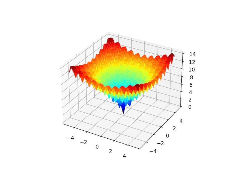
3D Surface Plot of the Ackley Multimodal Function
We can apply the basin hopping algorithm to the Ackley objective function.
In this case, we will start the search using a random point drawn from the input domain between -5 and 5.
|
1 2 3 |
... # define the starting point as a random sample from the domain pt = r_min + rand(2) * (r_max - r_min) |
We will use a step size of 0.5, 200 iterations, and the default local search algorithm. This configuration was chosen after a little trial and error.
|
1 2 3 |
... # perform the basin hopping search result = basinhopping(objective, pt, stepsize=0.5, niter=200) |
After the search is complete, it will report the status of the search and the number of iterations performed as well as the best result found with its evaluation.
|
1 2 3 4 5 6 7 8 |
... # summarize the result print('Status : %s' % result['message']) print('Total Evaluations: %d' % result['nfev']) # evaluate solution solution = result['x'] evaluation = objective(solution) print('Solution: f(%s) = %.5f' % (solution, evaluation)) |
Tying this together, the complete example of applying basin hopping to the Ackley objective function is listed below.
|
1 2 3 4 5 6 7 8 9 10 11 12 13 14 15 16 17 18 19 20 21 22 23 24 25 26 27 |
# basin hopping global optimization for the ackley multimodal objective function from scipy.optimize import basinhopping from numpy.random import rand from numpy import exp from numpy import sqrt from numpy import cos from numpy import e from numpy import pi # objective function def objective(v): x, y = v return -20.0 * exp(-0.2 * sqrt(0.5 * (x**2 + y**2))) - exp(0.5 * (cos(2 * pi * x) + cos(2 * pi * y))) + e + 20 # define range for input r_min, r_max = -5.0, 5.0 # define the starting point as a random sample from the domain pt = r_min + rand(2) * (r_max - r_min) # perform the basin hopping search result = basinhopping(objective, pt, stepsize=0.5, niter=200) # summarize the result print('Status : %s' % result['message']) print('Total Evaluations: %d' % result['nfev']) # evaluate solution solution = result['x'] evaluation = objective(solution) print('Solution: f(%s) = %.5f' % (solution, evaluation)) |
Running the example executes the optimization, then reports the results.
Note: Your results may vary given the stochastic nature of the algorithm or evaluation procedure, or differences in numerical precision. Consider running the example a few times and compare the average outcome.
In this case, we can see that the algorithm located the optima with inputs very close to zero and an objective function evaluation that is practically zero.
We can see that 200 iterations of the algorithm resulted in 86,020 function evaluations.
|
1 2 3 |
Status: ['requested number of basinhopping iterations completed successfully'] Total Evaluations: 86020 Solution: f([ 5.29778873e-10 -2.29022817e-10]) = 0.00000 |
Multimodal Optimization With Multiple Global Optima
The Himmelblau function is an example of an objective function that has multiple global optima.
Specifically, it has four optima and each has the same objective function evaluation. It is a two-dimensional objective function that has a global optima at [3.0, 2.0], [-2.805118, 3.131312], [-3.779310, -3.283186], [3.584428, -1.848126].
This means each run of a global optimization algorithm may find a different global optima.
The example below implements the Himmelblau and creates a three-dimensional surface plot to give an intuition for the objective function.
|
1 2 3 4 5 6 7 8 9 10 11 12 13 14 15 16 17 18 19 20 21 22 23 24 25 |
# himmelblau multimodal test function from numpy import arange from numpy import meshgrid from matplotlib import pyplot from mpl_toolkits.mplot3d import Axes3D # objective function def objective(x, y): return (x**2 + y - 11)**2 + (x + y**2 -7)**2 # define range for input r_min, r_max = -5.0, 5.0 # sample input range uniformly at 0.1 increments xaxis = arange(r_min, r_max, 0.1) yaxis = arange(r_min, r_max, 0.1) # create a mesh from the axis x, y = meshgrid(xaxis, yaxis) # compute targets results = objective(x, y) # create a surface plot with the jet color scheme figure = pyplot.figure() axis = figure.gca(projection='3d') axis.plot_surface(x, y, results, cmap='jet') # show the plot pyplot.show() |
Running the example creates the surface plot of the Himmelblau function showing the four global optima as dark blue basins.
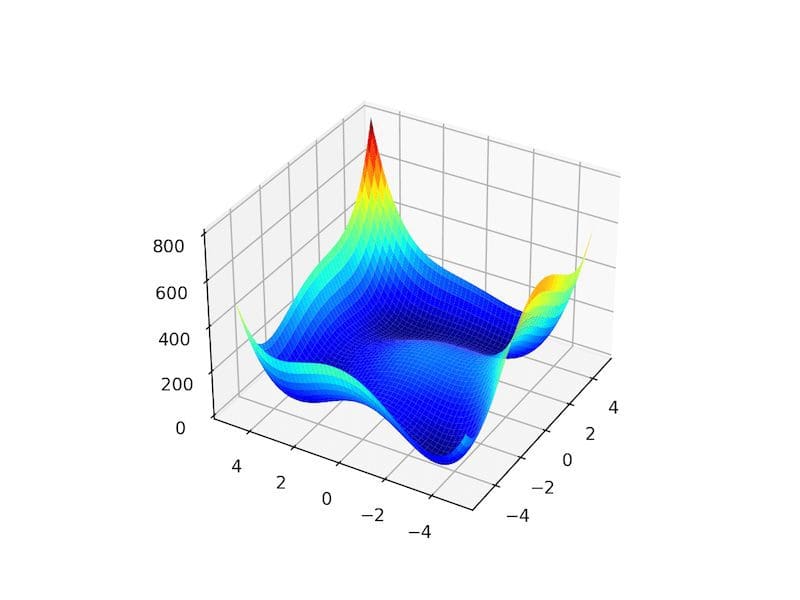
3D Surface Plot of the Himmelblau Multimodal Function
We can apply the basin hopping algorithm to the Himmelblau objective function.
As in the previous example, we will start the search using a random point drawn from the input domain between -5 and 5.
We will use a step size of 0.5, 200 iterations, and the default local search algorithm. At the end of the search, we will report the input for the best located optima,
|
1 2 3 4 5 6 7 8 9 10 11 12 13 14 15 16 17 18 19 20 21 22 |
# basin hopping global optimization for the himmelblau multimodal objective function from scipy.optimize import basinhopping from numpy.random import rand # objective function def objective(v): x, y = v return (x**2 + y - 11)**2 + (x + y**2 -7)**2 # define range for input r_min, r_max = -5.0, 5.0 # define the starting point as a random sample from the domain pt = r_min + rand(2) * (r_max - r_min) # perform the basin hopping search result = basinhopping(objective, pt, stepsize=0.5, niter=200) # summarize the result print('Status : %s' % result['message']) print('Total Evaluations: %d' % result['nfev']) # evaluate solution solution = result['x'] evaluation = objective(solution) print('Solution: f(%s) = %.5f' % (solution, evaluation)) |
Running the example executes the optimization, then reports the results.
Want to Get Started With Ensemble Learning?
Take my free 7-day email crash course now (with sample code).
Click to sign-up and also get a free PDF Ebook version of the course.
In this case, we can see that the algorithm located an optima at about [3.0, 2.0].
We can see that 200 iterations of the algorithm resulted in 7,660 function evaluations.
|
1 2 3 |
Status : ['requested number of basinhopping iterations completed successfully'] Total Evaluations: 7660 Solution: f([3. 1.99999999]) = 0.00000 |
If we run the search again, we may expect a different global optima to be located.
For example, below, we can see an optima located at about [-2.805118, 3.131312], different from the previous run.
|
1 2 3 |
Status : ['requested number of basinhopping iterations completed successfully'] Total Evaluations: 7636 Solution: f([-2.80511809 3.13131252]) = 0.00000 |
Further Reading
This section provides more resources on the topic if you are looking to go deeper.
Papers
- Global Optimization by Basin-Hopping and the Lowest Energy Structures of Lennard-Jones Clusters Containing up to 110 Atoms, 1997.
- Basin Hopping With Occasional Jumping, 2004.
Books
APIs
Articles
Summary
In this tutorial, you discovered the basin hopping global optimization algorithm.
Specifically, you learned:
- Basin hopping optimization is a global optimization that uses random perturbations to jump basins, and a local search algorithm to optimize each basin.
- How to use the basin hopping optimization algorithm API in python.
- Examples of using basin hopping to solve global optimization problems with multiple optima.
Do you have any questions?
Ask your questions in the comments below and I will do my best to answer.
Get a Handle on Modern Optimization Algorithms!

Develop Your Understanding of Optimization
...with just a few lines of python code
Discover how in my new Ebook:
Optimization for Machine Learning
It provides self-study tutorials with full working code on:
Gradient Descent, Genetic Algorithms, Hill Climbing, Curve Fitting, RMSProp, Adam,
and much more...
")


Dear Dr Jason,
In the second last piece of code you have the following import line
I noticed that the Axes3D is not invoked.
So I commented-out the line
Conclusion: no errors produced in the program
I presume then that Axes3D was not necessary since the ‘3d’ parameter was set already in
Thank you,
Anthony of Sydney
Thanks.
Dear Dr Jason,
In the last example, you mentioned the basinhopping function to find a global minimum.
Is there a function to find a global maximum? Reason for asking is I did a dir(scipy.optimize) and could not find an intuitive name for the opposite of basinhopping to find a global maximum.
Thank you,
Anthony of Sydney
Yes, you can invert a maximizing problem by adding a negative sign to the results from the cost function to give a minimization problem.
Dear Dr Jason,
I attempted “adding a negative sign to the results”:
The following results:
All I want to do is find the global maximum.
Thank you,
Anthony of Sydney
You would add a negative sign to the result returned from the objective() function, e.g. the last line of the function.
Dear Dr Jason,
Thank you for this.
Result of changing the polarity of the objective function:
I learned one thing:
The objective function returned the negative of the function in order to ‘find’ the global maximum:
BUT one thing that is not clear is how did you pass v into the objective function when the code did not specify what v is in when objective function was invoked in the basinhopping function?
Thank you,
Anthony of Sydney
The function is searching the domain for v – that is the definition of than optimization problem.
Dear Dr Jason,
Thank you for that.
So how does v get passed from the objective function in the following when you did not declare NOR assign v:
Thank you,
Anthony of Sydney
The optimization algorithm generates candidates of “v” that are evaluated by our objective function.
Dear Dr Jason,
Thank you for your answer and patience.
I did an ‘experiment’ with the objective’s parameter v and replaced with something else.
Conclusions:
* It seems that the parameter is used INTERNALLY by the basinhopping function without you having to explicitly pass.
* The objective’s parameter whether you call it v or boobooboo is of type ndarray:
– the variable result is of type scipy.optimize.optimize.OptimizeResult
– result[‘x’] returns an ndarray of the optimized value for x and y.
– result[‘x’] is passed into objective(v) or objective(boobooboo) to return a result of z.
Thank you, again for your time and patience
Anthony of Sydney
Yes.
Dear Dr Jason,
I made a program which combines basinhopping and displaying the 3d (x,y,z) of the function.
It works.
It requires the using the objective function twice. (i) first the basinhopping function does not need x and y, and for (ii) printing the graphics, requires a separate setup of the x, y and z
Conclusions:
* comparing the computed x, y and z, with the graph we find that the minimum occurs at
Solution: f([4.41865299e-10 1.35549800e-10]) = 0.00000
* When using the graph, the minimum occurs at (0,0) = 0.
Recall:
* To evaluate objective in basinhopping, the function generates the internal x and y.
* To print the 3d objective function requires you to generate the x and y, feed the x, y into the objective function by:
– making a meshgrid v = np.array([x,y])
– plugging the meshgrid into objective function objective(v)
– plot the data.
Thank you,
Anthony of Sydney.
Thanks for sharing!
Dear Dr Jason,
In ‘my’ comment above, I wanted to find the global maximum using the working code above to find the global minimum.
To find the global maximum, I inverted the return value of the original objective function.
As expected the 3D plot of x, y, z was inverted.
BUT:
* repeating the program a number of times, produced the same result:
most of the time, z = f(x,y) = -22.35040, occasionally, z = f(x,y) was -16.
* even then, on VISUAL INSPECTION of the actual graph, the expected value is z = f(x,y) = -6 ..
THE CODE:
* there was no change between the code presented in the previous comment and the code presented in this comment, but for the change in sign in the objective function.
SUMMARY:
* Changing the sign of the results of the objective function is supposed to help us determine the global maximum.
* Despite repeated running of the code, z = f(x,y) = -22.35040 BUT DID NOT on visual inspection of the 3D graph look like like the expected value = z = f(x,y) = f(0,0) = -6.
Thank you,
Anthony of Sydney
Perhaps a bug was introduced?
Perhaps the function was sufficiently changed to define a new optima?
…
Dear Dr Jason,
Thank you for the reply.
From your reply, I don’t see how a bug was introduced when it is a “copy” of the program only with a change in the sign of the return of the objective function objective = z = f(x,y)
However, my gut feel is that the “…function was sufficiently changed to define a new optima….”
If there is a function that calculates a global minimum, there should be an equivalent that finds a global maximum.
In the calculus, we don’t only calculate the minimum of a function, but it may be “necessary” to also calculate a global maximum.
Question: surely there must be a method to calculate the maximum of a function? Maybe it is not from the scipy.optimize module.
Again thank you for time and patience,
Anthony of Sydney
I was guessing at the cause of the fault, perhaps I missed some good guesses.
The typical method used on the domain of optimization is to invert (change the sign) the function rather than change the algorithm.
Dear Dr Jason,
I may come to it at a later time.
Where you say that the “…typical m ethod used on the domain….change the sign…(of) the function….”
That has been demonstrated before where on inspection of the graph, the negatived objective function did not return the maximum depicted in the graphic.
I will give it a break and resume at a later time,
Thanks for your time and patience,
Anthony of Sydney
Hey Dr. Jason, Thanks for sharing.
I am wondering if it is possible to use machine learning prediction models, i.e. a random forest regressor model as the objection function? with a goal to optimize controllable input features to the machine learning model.
Thank you!
Hi CC…this is possible and is a common practice when performing hyperparameter optimization.
Thank you for the quick tutorial. One thing I haven’t figured out yet is how to control the tolerance for success. For example, if I want a successful iteration when the objective function gets to 0.1 is there an input variable for that (i.e., tol = 0.1). The other way around I thought would be to input some weighting on the objective function via “args”… Thoughts?
Hi Scott…You are very welcome! The following resource may add clarity:
https://datascience.stackexchange.com/questions/49255/how-to-make-scipy-optimize-basinhopping-find-the-global-optimal-point