Build And Understand a Vector Database From Scratch in 10 Easy Steps

In this article, you will learn how a vector database works under the hood by building one from scratch in ten incremental steps using Python and NumPy.

Topics we will cover include:

• How documents are encoded into fixed-size vectors and searched by meaning rather than by keyword.
• How to add metadata filtering, input validation, and persistence to a minimal vector database.
• How brute-force cosine similarity scales with corpus size, and when to consider approximate indexing.

Introducing Vector Databases

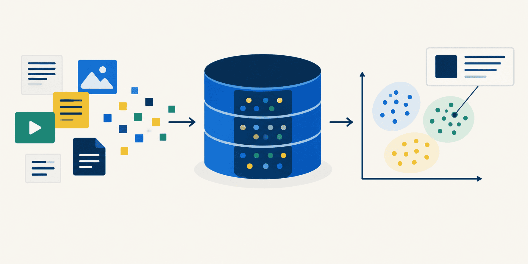
A vector database answers questions by meaning rather than by keyword. It operates by turning every document into a vector of numbers and then finding the numbers that point in a similar direction to your query (which has also been turned into a vector of numbers). This tutorial will demonstrate how to build a working vector database of your very own, through ten steps that each demonstrate one atomic idea. To follow along, create an empty script and name it something clever like tutorial.py. Append each step’s code to the script as you go and re-run it after you make sense of the commentary. The resulting output should make sense at that point. Nothing here needs a GPU or an API key; one small model downloads on the first run, and everything after that is plain NumPy.

Step 1: Setup

You need three files from this repository in your working directory: vector_db.py is the actual database which, yes, is already built for you… but the real magic is the understanding of the code and the interaction with it using the code herein. The good news is, once you go through this tutorial and understand the code, recreating the vector database on your own is nearly trivial. corpus.py contains 25 simulated sample documents and their topic tags. test.py is the test suite, only here to make you feel safe and secure that the vector database works properly as implemented, which you can verify by running at any point with python test.py.

Install the two dependencies:

Now start your tutorial.py file with the imports and two small display helpers. show() prints a list of search results as score, topic, document (relied upon later). header() just labels each section so the growing script’s output stays readable.

Running the script now produces no output. This is what we want; nothing has been called yet.

Step 2: Building the Index

Creating a VectorDB loads the embedding model, and add() encodes every document into a vector and stores it.

Output:

Note that the index size does not depend on how long the documents are. Every document, whether a six-word sentence or a six-page essay, becomes the same 384 numbers at 4 bytes each: 1,536 bytes, flat. That is fixed, and is what makes a vector index predictable to size and cheap to scan.

Step 3: A First Search

Output:

The top hit shares exactly one word with the query (“cell”) and the runner-up shares none at all. A keyword index would have ranked these very differently, if it found them at all.

Step 4: Searching Without Sharing a Single Word

Output:

This is the whole point of the exercise. Neither query shares any word with the documents it retrieves; no instances of “loaf”, “sour”, nor “superhero” appear anywhere in the corpus. The match is on meaning.

Step 5: Reading The Scores

header("5. Reading the scores") query = "the best way to change a tyre" print(f' query: "{query}"\n') show(db.search(query, k=3))

1 2 3 4 5

header("5. Reading the scores")   query = "the best way to change a tyre" print(f'  query: "{query}"\n') show(db.search(query, k=3))

Output:

5. Reading the scores ───────────────────── query: "the best way to change a tyre" +0.111 [ml ] Transformers replaced recurrent networks for most sequence tasks. +0.096 [comics ] Like Peter Parker's cells constantly regenerating thanks to his... +0.068 [ml ] The self-attention mechanism in transformers allows each token ...

1 2 3 4 5 6 7

5. Reading the scores ─────────────────────   query: "the best way to change a tyre"     +0.111  [ml     ]  Transformers replaced recurrent networks for most sequence tasks.   +0.096  [comics ]  Like Peter Parker's cells constantly regenerating thanks to his...   +0.068  [ml     ]  The self-attention mechanism in transformers allows each token ...

A vector search always returns k results, even when the corpus holds nothing relevant; it simply ranks what it has. The score is the only signal of whether an answer is any good: compare the +0.111 here against the +0.630 in step 4. In production you would set a floor and return nothing below it.

Step 6: Narrowing Results with Metadata

Every document was added with a {"topic": ...} dict. The where argument keeps only the documents whose metadata matches on every key given.

Output:

The corpus contains a deliberate trap: a comics document about Thor’s “mitochondria-rich muscle fibres” that is a genuinely good vector match for a biology question. Filtering is how you rule it the match — similarity alone cannot, because by meaning it really is similar.

Step 7: A Filter Narrower Than k

Output:

Only one document is tagged music, so asking for 5 returns 1. Results are filtered before they are ranked, meaning that a non-matching document can never be padded into the list just to reach k.

Step 8: Guard Rails

Output:

add() keeps documents, metadata and vectors in lockstep. Both of the above mistakes are easy to make and would silently corrupt an index if not caught. A bare string is iterable, so docs.extend("hi") would append “h” and “i” as two separate documents, and the model returned a single vector.

Step 9: Saving and Loading

Output:

The vectors go to .npy because it is compact and loads without parsing. The text and metadata go to .json so you can open the file and read it. load() refuses an index built by a different model. This is important because embeddings only mean something relative to the model that produced them; mixing them would not be a little bit “off,” it would be confident nonsense.

Step 10: How This Scales

Twenty-five documents are too few to measure, so this step also times a synthetic corpus of random vectors. They score meaningless results, but the computational cost matches a real world scenario.

Output:

At 25 documents, embedding the query is essentially the entire computation, since the search itself is too fast to measure. Note that milliseconds() discards one warm-up run; the first call to a NumPy matrix routine spins up its internal thread pool, which can take more time than the actual work itself, with a result of making a small corpus look slower than a large one.

Two things are worth pointing out in the results table above:

1. Both columns grow linearly; nothing here is clever, it simply touches every row.
2. Past ~100,000 rows the sort starts to outgrow the scan. At a million documents the scan takes about 25 ms and the full sort about 90 ms. That is the point where it pays to stop sorting everything (np.argpartition finds the top k in about 10 ms). Not far beyond this you will find the point where you reach for a real approximate index (HNSW, IVF) and trade a little accuracy for speed.

Wrapping Up

Every step here rests on a single idea: scale each embedding to length 1, and a plain dot product becomes cosine similarity. Ranking an entire corpus is then one matrix multiply. Everything else you added along the way — from metadata filters, saving and loading, the guard rails on add() — is bookkeeping that keeps documents, metadata and vectors in lockstep, so that the multiplication remains meaningful.

The big takeaway — beyond the simplicity and elegance behind the implementation of a vector database’s core functionality — is that the design does not change between 25 documents and 25 million; only the index structure underneath it does. This is, not surprisingly, precisely what the managed vector databases are selling.

For more information on vector databases from different points of view, check out these Machine Learning Mastery resources:

• Understanding RAG Part VII: Vector Databases & Indexing Strategies by Iván Palomares Carrascosa
• Vector Databases Explained in 3 Levels of Difficulty by Bala Priya C
• The Complete Guide to Vector Databases for Machine Learning by Bala Priya C