Visualizing the vanishing gradient problem

Deep learning was a recent invention. Partially, it is due to improved computation power that allows us to use more layers of perceptrons in a neural network. But at the same time, we can train a deep network only after we know how to work around the vanishing gradient problem.

In this tutorial, we visually examine why vanishing gradient problem exists.

After completing this tutorial, you will know

• What is a vanishing gradient
• Which configuration of neural network will be susceptible to vanishing gradient
• How to run manual training loop in Keras
• How to extract weights and gradients from Keras model

Let’s get started

Visualizing the vanishing gradient problem
Photo by Alisa Anton, some rights reserved.

Tutorial overview

This tutorial is divided into 5 parts; they are:

1. Configuration of multilayer perceptron models
2. Example of vanishing gradient problem
3. Looking at the weights of each layer
4. Looking at the gradients of each layer
5. The Glorot initialization

Configuration of multilayer perceptron models

Because neural networks are trained by gradient descent, people believed that a differentiable function is required to be the activation function in neural networks. This caused us to conventionally use sigmoid function or hyperbolic tangent as activation.

For a binary classification problem, if we want to do logistic regression such that 0 and 1 are the ideal output, sigmoid function is preferred as it is in this range:
$$
\sigma(x) = \frac{1}{1+e^{-x}}
$$
and if we need sigmoidal activation at the output, it is natural to use it in all layers of the neural network. Additionally, each layer in a neural network has a weight parameter. Initially, the weights have to be randomized and naturally we would use some simple way to do it, such as using uniform random or normal distribution.

Example of vanishing gradient problem

To illustrate the problem of vanishing gradient, let’s try with an example. Neural network is a nonlinear function. Hence it should be most suitable for classification of nonlinear dataset. We make use of scikit-learn’s make_circle() function to generate some data:

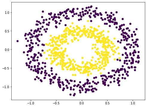
This is not difficult to classify. A naive way is to build a 3-layer neural network, which can give a quite good result:

Note that we used rectified linear unit (ReLU) in the hidden layer above. By default, the dense layer in Keras will be using linear activation (i.e. no activation) which mostly is not useful. We usually use ReLU in modern neural networks. But we can also try the old school way as everyone does two decades ago:

The accuracy is much worse. It turns out, it is even worse by adding more layers (at least in my experiment):

Your result may vary given the stochastic nature of the training algorithm. You may see the 5-layer sigmoidal network performing much worse than 3-layer or not. But the idea here is you can’t get back the high accuracy as we can achieve with rectified linear unit activation by merely adding layers.

Looking at the weights of each layer

Shouldn’t we get a more powerful neural network with more layers?

Yes, it should be. But it turns out as we adding more layers, we triggered the vanishing gradient problem. To illustrate what happened, let’s see how are the weights look like as we trained our network.

In Keras, we are allowed to plug-in a callback function to the training process. We are going create our own callback object to intercept and record the weights of each layer of our multilayer perceptron (MLP) model at the end of each epoch.

We derive the Callback class and define the on_epoch_end() function. This class will need the created model to initialize. At the end of each epoch, it will read each layer and save the weights into numpy array.

For the convenience of experimenting different ways of creating a MLP, we make a helper function to set up the neural network model:

We deliberately create a neural network with 4 hidden layers so we can see how each layer respond to the training. We will vary the activation function of each hidden layer as well as the weight initialization. To make things easier to tell, we are going to name each layer instead of letting Keras to assign a name. The input is a coordinate on the xy-plane hence the input shape is a vector of 2. The output is binary classification. Therefore we use sigmoid activation to make the output fall in the range of 0 to 1.

Then we can compile() the model to provide the evaluation metrics and pass on the callback in the fit() call to train the model:

Here we create the neural network by calling make_mlp() first. Then we set up our callback object. Since the weights of each layer in the neural network are initialized at creation, we deliberately call the callback function to remember what they are initialized to. Then we call the compile() and fit() from the model as usual, with the callback object provided.

After we fit the model, we can evaluate it with the entire dataset:

Here it means the log-loss is 0.665 and the accuracy is 0.588 for this model of having all layers using sigmoid activation.

What we can further look into is how the weight behaves along the iterations of training. All the layers except the first and the last are having their weight as a 5×5 matrix. We can check the mean and standard deviation of the weights to get a sense of how the weights look like:

This results in the following figure: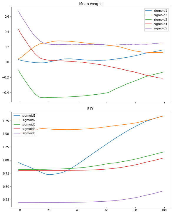

We see the mean weight moved quickly only in first 10 iterations or so. Only the weights of the first layer getting more diversified as its standard deviation is moving up.

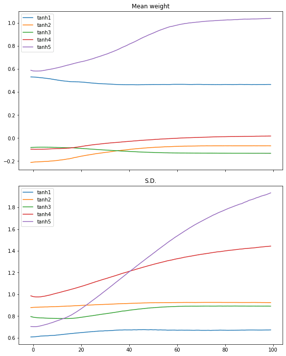
We can restart with the hyperbolic tangent (tanh) activation on the same process:

The log-loss and accuracy are both improved. If we look at the plot, we don’t see the abrupt change in the mean and standard deviation in the weights but instead, that of all layers are slowly converged.

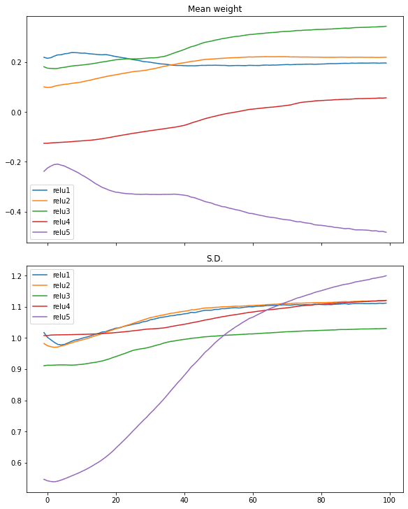
Similar case can be seen in ReLU activation:

Looking at the gradients of each layer

We see the effect of different activation function in the above. But indeed, what matters is the gradient as we are running gradient decent during training. The paper by Xavier Glorot and Yoshua Bengio, “Understanding the difficulty of training deep feedforward neural networks”, suggested to look at the gradient of each layer in each training iteration as well as the standard deviation of it.

Bradley (2009) found that back-propagated gradients were smaller as one moves from the output layer towards the input layer, just after initialization. He studied networks with linear activation at each layer, finding that the variance of the back-propagated gradients decreases as we go backwards in the network

— “Understanding the difficulty of training deep feedforward neural networks” (2010)

To understand how the activation function related to the gradient as perceived during training, we need to run the training loop manually.

In Tensorflow-Keras, a training loop can be run by turning on the gradient tape, and then make the neural network model produce an output, which afterwards we can obtain the gradient by automatic differentiation from the gradient tape. Subsequently we can update the parameters (weights and biases) according to the gradient descent update rule.

Because the gradient is readily obtained in this loop, we can make a copy of it. The following is how we implement the training loop and at the same time, keep a copy of the gradients:

The key in the function above is the nested for-loop. In which, we launch tf.GradientTape() and pass in a batch of data to the model to get a prediction, which is then evaluated using the loss function. Afterwards, we can pull out the gradient from the tape by comparing the loss with the trainable weight from the model. Next, we update the weights using the optimizer, which will handle the learning weights and momentums in the gradient descent algorithm implicitly.

As a refresh, the gradient here means the following. For a loss value $L$ computed and a layer with weights $W=[w_1, w_2, w_3, w_4, w_5]$ (e.g., on the output layer) then the gradient is the matrix

$$
\frac{\partial L}{\partial W} = \Big[\frac{\partial L}{\partial w_1}, \frac{\partial L}{\partial w_2}, \frac{\partial L}{\partial w_3}, \frac{\partial L}{\partial w_4}, \frac{\partial L}{\partial w_5}\Big]
$$

But before we start the next iteration of training, we have a chance to further manipulate the gradient: We match the gradient with the weights, to get the name of each, then save a copy of the gradient as numpy array. We sample the weight and loss only once per epoch, but you can change that to sample in a higher frequency.

With these, we can plot the gradient across epochs. In the following, we create the model (but not calling compile() because we would not call fit() afterwards) and run the manual training loop, then plot the gradient as well as the standard deviation of the gradient:

It reported a weak classification result:

and the plot we obtained shows vanishing gradient:

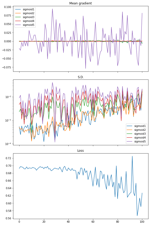
From the plot, the loss is not significantly decreased. The mean of gradient (i.e., mean of all elements in the gradient matrix) has noticeable value only for the last layer while all other layers are virtually zero. The standard deviation of the gradient is at the level of between 0.01 and 0.001 approximately.

Repeat this with tanh activation, we see a different result, which explains why the performance is better:

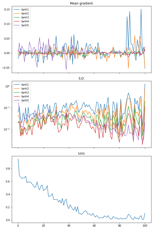
From the plot of the mean of the gradients, we see the gradients from every layer are wiggling equally. The standard deviation of the gradient are also an order of magnitude larger than the case of sigmoid activation, at around 0.1 to 0.01.

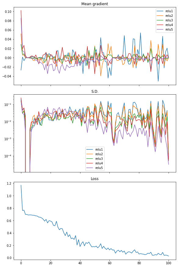
Finally, we can also see the similar in rectified linear unit (ReLU) activation. And in this case the loss dropped quickly, hence we see it as the more efficient activation to use in neural networks:

The following is the complete code:

The Glorot initialization

We didn’t demonstrate in the code above, but the most famous outcome from the paper by Glorot and Bengio is the Glorot initialization. Which suggests to initialize the weights of a layer of the neural network with uniform distribution:

The normalization factor may therefore be important when initializing deep networks because of the multiplicative effect through layers, and we suggest the following initialization procedure to approximately satisfy our objectives of maintaining activation variances and back-propagated gradients variance as one moves up or down the network. We call it the normalized initialization:
$$
W \sim U\Big[-\frac{\sqrt{6}}{\sqrt{n_j+n_{j+1}}}, \frac{\sqrt{6}}{\sqrt{n_j+n_{j+1}}}\Big]
$$

— “Understanding the difficulty of training deep feedforward neural networks” (2010)

This is derived from the linear activation on the condition that the standard deviation of the gradient is keeping consistent across the layers. In the sigmoid and tanh activation, the linear region is narrow. Therefore we can understand why ReLU is the key to workaround the vanishing gradient problem. Comparing to replacing the activation function, changing the weight initialization is less pronounced in helping to resolve the vanishing gradient problem. But this can be an exercise for you to explore to see how this can help improving the result.

Further readings

The Glorot and Bengio paper is available at:

• “Understanding the difficulty of training deep feedforward neural networks”, by Xavier Glorot and Yoshua Bengio, 2010.
  (https://proceedings.mlr.press/v9/glorot10a/glorot10a.pdf)

The vanishing gradient problem is well known enough in machine learning that many books covered it. For example,

• Deep Learning, by Ian Goodfellow, Yoshua Bengio, and Aaron Courville, 2016.
  (https://www.amazon.com/dp/0262035618)

Previously we have posts about vanishing and exploding gradients:

• How to fix vanishing gradients using the rectified linear activation function
• Exploding gradients in neural networks

You may also find the following documentation helpful to explain some syntax we used above:

• Writings a training loop from scratch in Keras: https://keras.io/guides/writing_a_training_loop_from_scratch/
• Writing your own callbacks in Keras: https://keras.io/guides/writing_your_own_callbacks/

Summary

In this tutorial, you visually saw how a rectified linear unit (ReLU) can help resolving the vanishing gradient problem.

Specifically, you learned:

• How the problem of vanishing gradient impact the performance of a neural network
• Why ReLU activation is the solution to vanishing gradient problem
• How to use a custom callback to extract data in the middle of training loop in Keras
• How to write a custom training loop
• How to read the weight and gradient from a layer in the neural network

Develop Better Deep Learning Models Today!

Train Faster, Reduce Overftting, and Ensembles

...with just a few lines of python code

Discover how in my new Ebook:
Better Deep Learning

It provides self-study tutorials on topics like:
weight decay, batch normalization, dropout, model stacking and much more...

Bring better deep learning to your projects!

Skip the Academics. Just Results.

See What's Inside