Weight Regularization with LSTM Networks for Time Series Forecasting

By Jason Brownlee on August 28, 2020 in Deep Learning for Time Series 65

Long Short-Term Memory (LSTM) models are a recurrent neural network capable of learning sequences of observations.

This may make them a network well suited to time series forecasting.

An issue with LSTMs is that they can easily overfit training data, reducing their predictive skill.

Weight regularization is a technique for imposing constraints (such as L1 or L2) on the weights within LSTM nodes. This has the effect of reducing overfitting and improving model performance.

In this tutorial, you will discover how to use weight regularization with LSTM networks and design experiments to test for its effectiveness for time series forecasting.

After completing this tutorial, you will know:

How to design a robust test harness for evaluating LSTM networks for time series forecasting.
How to design, execute, and interpret the results from using bias weight regularization with LSTMs.
How to design, execute, and interpret the results from using input and recurrent weight regularization with LSTMs.

Kick-start your project with my new book Deep Learning for Time Series Forecasting, including step-by-step tutorials and the Python source code files for all examples.

Let’s get started.

Updated Apr/2019: Updated the link to dataset.

How to Use Weight Regularization with LSTM Networks for Time Series Forecasting
Photo by Julian Fong, some rights reserved.

Tutorial Overview

This tutorial is broken down into 6 parts. They are:

Shampoo Sales Dataset
Experimental Test Harness
Bias Weight Regularization
Input Weight Regularization
Recurrent Weight Regularization
Review of Results

Environment

This tutorial assumes you have a Python SciPy environment installed. You can use either Python 2 or 3 with this example.

This tutorial assumes you have Keras v2.0 or higher installed with either the TensorFlow or Theano backend.

This tutorial also assumes you have scikit-learn, Pandas, NumPy, and Matplotlib installed.

If you need help setting up your Python environment, see this post:

How to Setup a Python Environment for Machine Learning and Deep Learning with Anaconda

Next, let’s take a look at a standard time series forecasting problem that we can use as context for this experiment.

Need help with Deep Learning for Time Series?

Take my free 7-day email crash course now (with sample code).

Click to sign-up and also get a free PDF Ebook version of the course.

Shampoo Sales Dataset

This dataset describes the monthly number of sales of shampoo over a 3-year period.

The units are a sales count and there are 36 observations. The original dataset is credited to Makridakis, Wheelwright, and Hyndman (1998).

Download the dataset.

The example below loads and creates a plot of the loaded dataset.

# load and plot dataset
from pandas import read_csv
from pandas import datetime
from matplotlib import pyplot
# load dataset
def parser(x):
	return datetime.strptime('190'+x, '%Y-%m')
series = read_csv('shampoo-sales.csv', header=0, parse_dates=[0], index_col=0, squeeze=True, date_parser=parser)
# summarize first few rows
print(series.head())
# line plot
series.plot()
pyplot.show()

# load and plot dataset

from pandas import read_csv

from pandas import datetime

from matplotlib import pyplot

# load dataset

def parser(x):

return datetime.strptime('190'+x, '%Y-%m')

series = read_csv('shampoo-sales.csv', header=0, parse_dates=[0], index_col=0, squeeze=True, date_parser=parser)

# summarize first few rows

print(series.head())

# line plot

series.plot()

pyplot.show()

Running the example loads the dataset as a Pandas Series and prints the first 5 rows.

Month
1901-01-01 266.0
1901-02-01 145.9
1901-03-01 183.1
1901-04-01 119.3
1901-05-01 180.3
Name: Sales, dtype: float64

Month

1901-01-01 266.0

1901-02-01 145.9

1901-03-01 183.1

1901-04-01 119.3

1901-05-01 180.3

Name: Sales, dtype: float64

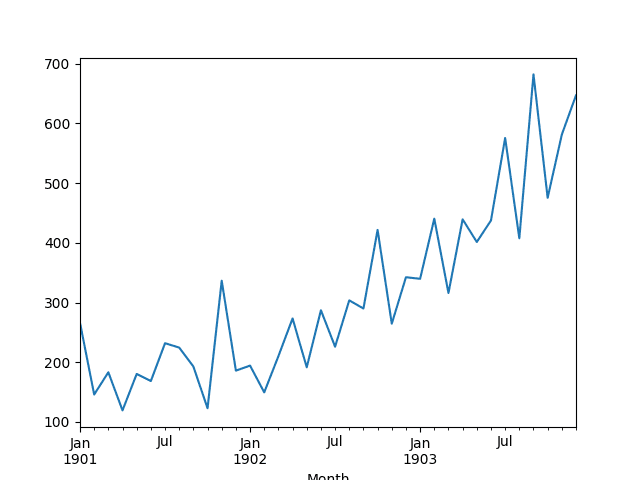
A line plot of the series is then created showing a clear increasing trend.

Line Plot of Shampoo Sales Dataset

Next, we will take a look at the model configuration and test harness used in the experiment.

Experimental Test Harness

This section describes the test harness used in this tutorial.

Data Split

We will split the Shampoo Sales dataset into two parts: a training and a test set.

The first two years of data will be taken for the training dataset and the remaining one year of data will be used for the test set.

Models will be developed using the training dataset and will make predictions on the test dataset.

The persistence forecast (naive forecast) on the test dataset achieves an error of 136.761 monthly shampoo sales. This provides a lower acceptable bound of performance on the test set.

Model Evaluation

A rolling-forecast scenario will be used, also called walk-forward model validation.

Each time step of the test dataset will be walked one at a time. A model will be used to make a forecast for the time step, then the actual expected value from the test set will be taken and made available to the model for the forecast on the next time step.

This mimics a real-world scenario where new Shampoo Sales observations would be available each month and used in the forecasting of the following month.

This will be simulated by the structure of the train and test datasets.

All forecasts on the test dataset will be collected and an error score calculated to summarize the skill of the model. The root mean squared error (RMSE) will be used as it punishes large errors and results in a score that is in the same units as the forecast data, namely monthly shampoo sales.

Data Preparation

Before we can fit a model to the dataset, we must transform the data.

The following three data transforms are performed on the dataset prior to fitting a model and making a forecast.

Transform the time series data so that it is stationary. Specifically, a lag=1 differencing to remove the increasing trend in the data.
Transform the time series into a supervised learning problem. Specifically, the organization of data into input and output patterns where the observation at the previous time step is used as an input to forecast the observation at the current timestep
Transform the observations to have a specific scale. Specifically, to rescale the data to values between -1 and 1.

These transforms are inverted on forecasts to return them into their original scale before calculating and error score.

LSTM Model

We will use a base stateful LSTM model with 1 neuron fit for 1000 epochs.

Ideally a batch size of 1 would be used for walk-foward validation. We will assume walk-forward validation and predict the whole year for speed. As such we can use any batch size that is divisble by the number of samples, in this case we will use a value of 4.

Ideally, more training epochs would be used (such as 1500), but this was truncated to 1000 to keep run times reasonable.

The model will be fit using the efficient ADAM optimization algorithm and the mean squared error loss function.

Experimental Runs

Each experimental scenario will be run 30 times and the RMSE score on the test set will be recorded from the end each run.

Let’s dive into the experiments.

Baseline LSTM Model

Let’s start-off with the baseline LSTM model.

The baseline LSTM model for this problem has the following configuration:

Lag inputs: 1
Epochs: 1000
Units in LSTM hidden layer: 3
Batch Size: 4
Repeats: 3

The complete code listing is provided below.

This code listing will be used as the basis for all following experiments, with only the changes to this code provided in subsequent sections.

from pandas import DataFrame
from pandas import Series
from pandas import concat
from pandas import read_csv
from pandas import datetime
from sklearn.metrics import mean_squared_error
from sklearn.preprocessing import MinMaxScaler
from keras.models import Sequential
from keras.layers import Dense
from keras.layers import LSTM
from keras.regularizers import L1L2
from math import sqrt
import matplotlib
# be able to save images on server
matplotlib.use('Agg')
from matplotlib import pyplot
import numpy

# date-time parsing function for loading the dataset
def parser(x):
	return datetime.strptime('190'+x, '%Y-%m')

# frame a sequence as a supervised learning problem
def timeseries_to_supervised(data, lag=1):
	df = DataFrame(data)
	columns = [df.shift(i) for i in range(1, lag+1)]
	columns.append(df)
	df = concat(columns, axis=1)
	return df

# create a differenced series
def difference(dataset, interval=1):
	diff = list()
	for i in range(interval, len(dataset)):
		value = dataset[i] - dataset[i - interval]
		diff.append(value)
	return Series(diff)

# invert differenced value
def inverse_difference(history, yhat, interval=1):
	return yhat + history[-interval]

# scale train and test data to [-1, 1]
def scale(train, test):
	# fit scaler
	scaler = MinMaxScaler(feature_range=(-1, 1))
	scaler = scaler.fit(train)
	# transform train
	train = train.reshape(train.shape[0], train.shape[1])
	train_scaled = scaler.transform(train)
	# transform test
	test = test.reshape(test.shape[0], test.shape[1])
	test_scaled = scaler.transform(test)
	return scaler, train_scaled, test_scaled

# inverse scaling for a forecasted value
def invert_scale(scaler, X, yhat):
	new_row = [x for x in X] + [yhat]
	array = numpy.array(new_row)
	array = array.reshape(1, len(array))
	inverted = scaler.inverse_transform(array)
	return inverted[0, -1]

# fit an LSTM network to training data
def fit_lstm(train, n_batch, nb_epoch, n_neurons):
	X, y = train[:, 0:-1], train[:, -1]
	X = X.reshape(X.shape[0], 1, X.shape[1])
	model = Sequential()
	model.add(LSTM(n_neurons, batch_input_shape=(n_batch, X.shape[1], X.shape[2]), stateful=True))
	model.add(Dense(1))
	model.compile(loss='mean_squared_error', optimizer='adam')
	for i in range(nb_epoch):
		model.fit(X, y, epochs=1, batch_size=n_batch, verbose=0, shuffle=False)
		model.reset_states()
	return model

# run a repeated experiment
def experiment(series, n_lag, n_repeats, n_epochs, n_batch, n_neurons):
	# transform data to be stationary
	raw_values = series.values
	diff_values = difference(raw_values, 1)
	# transform data to be supervised learning
	supervised = timeseries_to_supervised(diff_values, n_lag)
	supervised_values = supervised.values[n_lag:,:]
	# split data into train and test-sets
	train, test = supervised_values[0:-12], supervised_values[-12:]
	# transform the scale of the data
	scaler, train_scaled, test_scaled = scale(train, test)
	# run experiment
	error_scores = list()
	for r in range(n_repeats):
		# fit the model
		train_trimmed = train_scaled[2:, :]
		lstm_model = fit_lstm(train_trimmed, n_batch, n_epochs, n_neurons)
		# forecast test dataset
		test_reshaped = test_scaled[:,0:-1]
		test_reshaped = test_reshaped.reshape(len(test_reshaped), 1, 1)
		output = lstm_model.predict(test_reshaped, batch_size=n_batch)
		predictions = list()
		for i in range(len(output)):
			yhat = output[i,0]
			X = test_scaled[i, 0:-1]
			# invert scaling
			yhat = invert_scale(scaler, X, yhat)
			# invert differencing
			yhat = inverse_difference(raw_values, yhat, len(test_scaled)+1-i)
			# store forecast
			predictions.append(yhat)
		# report performance
		rmse = sqrt(mean_squared_error(raw_values[-12:], predictions))
		print('%d) Test RMSE: %.3f' % (r+1, rmse))
		error_scores.append(rmse)
	return error_scores

# configure the experiment
def run():
	# load dataset
	series = read_csv('shampoo-sales.csv', header=0, parse_dates=[0], index_col=0, squeeze=True, date_parser=parser)
	# configure the experiment
	n_lag = 1
	n_repeats = 30
	n_epochs = 1000
	n_batch = 4
	n_neurons = 3
	# run the experiment
	results = DataFrame()
	results['results'] = experiment(series, n_lag, n_repeats, n_epochs, n_batch, n_neurons)
	# summarize results
	print(results.describe())
	# save boxplot
	results.boxplot()
	pyplot.savefig('experiment_baseline.png')

# entry point
run()

100

101

102

103

104

105

106

107

108

109

110

111

112

113

114

115

116

117

118

119

120

121

122

123

124

125

126

127

128

129

130

131

132

133

134

135

from pandas import DataFrame

from pandas import Series

from pandas import concat

from pandas import read_csv

from pandas import datetime

from sklearn.metrics import mean_squared_error

from sklearn.preprocessing import MinMaxScaler

from keras.models import Sequential

from keras.layers import Dense

from keras.layers import LSTM

from keras.regularizers import L1L2

from math import sqrt

import matplotlib

# be able to save images on server

matplotlib.use('Agg')

from matplotlib import pyplot

import numpy

# date-time parsing function for loading the dataset

def parser(x):

return datetime.strptime('190'+x, '%Y-%m')

# frame a sequence as a supervised learning problem

def timeseries_to_supervised(data, lag=1):

df = DataFrame(data)

columns = [df.shift(i) for i in range(1, lag+1)]

columns.append(df)

df = concat(columns, axis=1)

return df

# create a differenced series

def difference(dataset, interval=1):

diff = list()

for i in range(interval, len(dataset)):

value = dataset[i] - dataset[i - interval]

diff.append(value)

return Series(diff)

# invert differenced value

def inverse_difference(history, yhat, interval=1):

return yhat + history[-interval]

# scale train and test data to [-1, 1]

def scale(train, test):

# fit scaler

scaler = MinMaxScaler(feature_range=(-1, 1))

scaler = scaler.fit(train)

# transform train

train = train.reshape(train.shape[0], train.shape[1])

train_scaled = scaler.transform(train)

# transform test

test = test.reshape(test.shape[0], test.shape[1])

test_scaled = scaler.transform(test)

return scaler, train_scaled, test_scaled

# inverse scaling for a forecasted value

def invert_scale(scaler, X, yhat):

new_row = [x for x in X] + [yhat]

array = numpy.array(new_row)

array = array.reshape(1, len(array))

inverted = scaler.inverse_transform(array)

return inverted[0, -1]

# fit an LSTM network to training data

def fit_lstm(train, n_batch, nb_epoch, n_neurons):

X, y = train[:, 0:-1], train[:, -1]

X = X.reshape(X.shape[0], 1, X.shape[1])

model = Sequential()

model.add(LSTM(n_neurons, batch_input_shape=(n_batch, X.shape[1], X.shape[2]), stateful=True))

model.add(Dense(1))

model.compile(loss='mean_squared_error', optimizer='adam')

for i in range(nb_epoch):

model.fit(X, y, epochs=1, batch_size=n_batch, verbose=0, shuffle=False)

model.reset_states()

return model

# run a repeated experiment

def experiment(series, n_lag, n_repeats, n_epochs, n_batch, n_neurons):

# transform data to be stationary

raw_values = series.values

diff_values = difference(raw_values, 1)

# transform data to be supervised learning

supervised = timeseries_to_supervised(diff_values, n_lag)

supervised_values = supervised.values[n_lag:,:]

# split data into train and test-sets

train, test = supervised_values[0:-12], supervised_values[-12:]

# transform the scale of the data

scaler, train_scaled, test_scaled = scale(train, test)

# run experiment

error_scores = list()

for r in range(n_repeats):

# fit the model

train_trimmed = train_scaled[2:, :]

lstm_model = fit_lstm(train_trimmed, n_batch, n_epochs, n_neurons)

# forecast test dataset

test_reshaped = test_scaled[:,0:-1]

test_reshaped = test_reshaped.reshape(len(test_reshaped), 1, 1)

output = lstm_model.predict(test_reshaped, batch_size=n_batch)

predictions = list()

for i in range(len(output)):

yhat = output[i,0]

X = test_scaled[i, 0:-1]

# invert scaling

yhat = invert_scale(scaler, X, yhat)

# invert differencing

yhat = inverse_difference(raw_values, yhat, len(test_scaled)+1-i)

# store forecast

predictions.append(yhat)

# report performance

rmse = sqrt(mean_squared_error(raw_values[-12:], predictions))

print('%d) Test RMSE: %.3f' % (r+1, rmse))

error_scores.append(rmse)

return error_scores

# configure the experiment

def run():

# load dataset

series = read_csv('shampoo-sales.csv', header=0, parse_dates=[0], index_col=0, squeeze=True, date_parser=parser)

# configure the experiment

n_lag = 1

n_repeats = 30

n_epochs = 1000

n_batch = 4

n_neurons = 3

# run the experiment

results = DataFrame()

results['results'] = experiment(series, n_lag, n_repeats, n_epochs, n_batch, n_neurons)

# summarize results

print(results.describe())

# save boxplot

results.boxplot()

pyplot.savefig('experiment_baseline.png')

# entry point

run()

Running the experiment prints summary statistics for the test RMSE for all repeats.

Note: Your results may vary given the stochastic nature of the algorithm or evaluation procedure, or differences in numerical precision. Consider running the example a few times and compare the average outcome.

We can see that on average, this model configuration achieves a test RMSE of about 92 monthly shampoo sales with a standard deviation of 5.

          results
count   30.000000
mean    92.842537
std      5.748456
min     81.205979
25%     89.514367
50%     92.030003
75%     96.926145
max    105.247117

results

count 30.000000

mean 92.842537

std 5.748456

min 81.205979

25% 89.514367

50% 92.030003

75% 96.926145

max 105.247117

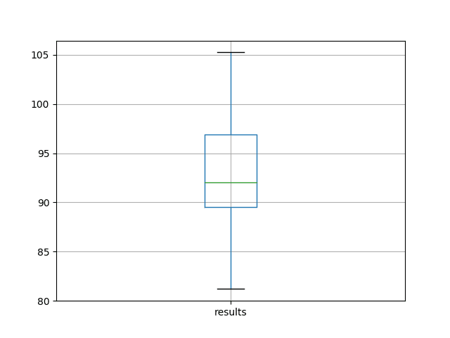
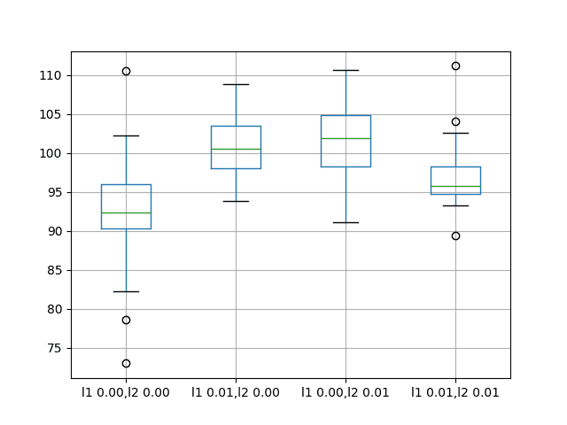
A box and whisker plot is also created from the distribution of test RMSE results and saved to a file.

The plot provides a clear depiction of the spread of the results, highlighting the middle 50% of values (the box) and the median (green line).

Box and Whisker Plot of Baseline Performance on the Shampoo Sales Dataset

Bias Weight Regularization

Weight regularization can be applied to the bias connection within the LSTM nodes.

In Keras, this is specified with a bias_regularizer argument when creating an LSTM layer. The regularizer is defined as an instance of the one of the L1, L2, or L1L2 classes.

More details here:

Keras Usage of Regularizers

In this experiment, we will compare L1, L2, and L1L2 with a default value of 0.01 against the baseline model. We can specify all configurations using the L1L2 class, as follows:

L1L2(0.0, 0.0) [e.g. baseline]
L1L2(0.01, 0.0) [e.g. L1]
L1L2(0.0, 0.01) [e.g. L2]
L1L2(0.01, 0.01) [e.g. L1L2 or elasticnet]

Below lists the updated fit_lstm(), experiment(), and run() functions for using bias weight regularization with LSTMs.

# fit an LSTM network to training data
def fit_lstm(train, n_batch, nb_epoch, n_neurons, reg):
	X, y = train[:, 0:-1], train[:, -1]
	X = X.reshape(X.shape[0], 1, X.shape[1])
	model = Sequential()
	model.add(LSTM(n_neurons, batch_input_shape=(n_batch, X.shape[1], X.shape[2]), stateful=True, bias_regularizer=reg))
	model.add(Dense(1))
	model.compile(loss='mean_squared_error', optimizer='adam')
	for i in range(nb_epoch):
		model.fit(X, y, epochs=1, batch_size=n_batch, verbose=0, shuffle=False)
		model.reset_states()
	return model

# run a repeated experiment
def experiment(series, n_lag, n_repeats, n_epochs, n_batch, n_neurons, reg):
	# transform data to be stationary
	raw_values = series.values
	diff_values = difference(raw_values, 1)
	# transform data to be supervised learning
	supervised = timeseries_to_supervised(diff_values, n_lag)
	supervised_values = supervised.values[n_lag:,:]
	# split data into train and test-sets
	train, test = supervised_values[0:-12], supervised_values[-12:]
	# transform the scale of the data
	scaler, train_scaled, test_scaled = scale(train, test)
	# run experiment
	error_scores = list()
	for r in range(n_repeats):
		# fit the model
		train_trimmed = train_scaled[2:, :]
		lstm_model = fit_lstm(train_trimmed, n_batch, n_epochs, n_neurons, reg)
		# forecast test dataset
		test_reshaped = test_scaled[:,0:-1]
		test_reshaped = test_reshaped.reshape(len(test_reshaped), 1, 1)
		output = lstm_model.predict(test_reshaped, batch_size=n_batch)
		predictions = list()
		for i in range(len(output)):
			yhat = output[i,0]
			X = test_scaled[i, 0:-1]
			# invert scaling
			yhat = invert_scale(scaler, X, yhat)
			# invert differencing
			yhat = inverse_difference(raw_values, yhat, len(test_scaled)+1-i)
			# store forecast
			predictions.append(yhat)
		# report performance
		rmse = sqrt(mean_squared_error(raw_values[-12:], predictions))
		print('%d) Test RMSE: %.3f' % (r+1, rmse))
		error_scores.append(rmse)
	return error_scores

# configure the experiment
def run():
	# load dataset
	series = read_csv('shampoo-sales.csv', header=0, parse_dates=[0], index_col=0, squeeze=True, date_parser=parser)
	# configure the experiment
	n_lag = 1
	n_repeats = 30
	n_epochs = 1000
	n_batch = 4
	n_neurons = 3
	regularizers = [L1L2(l1=0.0, l2=0.0), L1L2(l1=0.01, l2=0.0), L1L2(l1=0.0, l2=0.01), L1L2(l1=0.01, l2=0.01)]
	# run the experiment
	results = DataFrame()
	for reg in regularizers:
		name = ('l1 %.2f,l2 %.2f' % (reg.l1, reg.l2))
		results[name] = experiment(series, n_lag, n_repeats, n_epochs, n_batch, n_neurons, reg)
	# summarize results
	print(results.describe())
	# save boxplot
	results.boxplot()
	pyplot.savefig('experiment_reg_bias.png')

# fit an LSTM network to training data

def fit_lstm(train, n_batch, nb_epoch, n_neurons, reg):

X, y = train[:, 0:-1], train[:, -1]

X = X.reshape(X.shape[0], 1, X.shape[1])

model = Sequential()

model.add(LSTM(n_neurons, batch_input_shape=(n_batch, X.shape[1], X.shape[2]), stateful=True, bias_regularizer=reg))

model.add(Dense(1))

model.compile(loss='mean_squared_error', optimizer='adam')

for i in range(nb_epoch):

model.fit(X, y, epochs=1, batch_size=n_batch, verbose=0, shuffle=False)

model.reset_states()

return model

# run a repeated experiment

def experiment(series, n_lag, n_repeats, n_epochs, n_batch, n_neurons, reg):

# transform data to be stationary

raw_values = series.values

diff_values = difference(raw_values, 1)

# transform data to be supervised learning

supervised = timeseries_to_supervised(diff_values, n_lag)

supervised_values = supervised.values[n_lag:,:]

# split data into train and test-sets

train, test = supervised_values[0:-12], supervised_values[-12:]

# transform the scale of the data

scaler, train_scaled, test_scaled = scale(train, test)

# run experiment

error_scores = list()

for r in range(n_repeats):

# fit the model

train_trimmed = train_scaled[2:, :]

lstm_model = fit_lstm(train_trimmed, n_batch, n_epochs, n_neurons, reg)

# forecast test dataset

test_reshaped = test_scaled[:,0:-1]

test_reshaped = test_reshaped.reshape(len(test_reshaped), 1, 1)

output = lstm_model.predict(test_reshaped, batch_size=n_batch)

predictions = list()

for i in range(len(output)):

yhat = output[i,0]

X = test_scaled[i, 0:-1]

# invert scaling

yhat = invert_scale(scaler, X, yhat)

# invert differencing

yhat = inverse_difference(raw_values, yhat, len(test_scaled)+1-i)

# store forecast

predictions.append(yhat)

# report performance

rmse = sqrt(mean_squared_error(raw_values[-12:], predictions))

print('%d) Test RMSE: %.3f' % (r+1, rmse))

error_scores.append(rmse)

return error_scores

# configure the experiment

def run():

# load dataset

series = read_csv('shampoo-sales.csv', header=0, parse_dates=[0], index_col=0, squeeze=True, date_parser=parser)

# configure the experiment

n_lag = 1

n_repeats = 30

n_epochs = 1000

n_batch = 4

n_neurons = 3

regularizers = [L1L2(l1=0.0, l2=0.0), L1L2(l1=0.01, l2=0.0), L1L2(l1=0.0, l2=0.01), L1L2(l1=0.01, l2=0.01)]

# run the experiment

results = DataFrame()

for reg in regularizers:

name = ('l1 %.2f,l2 %.2f' % (reg.l1, reg.l2))

results[name] = experiment(series, n_lag, n_repeats, n_epochs, n_batch, n_neurons, reg)

# summarize results

print(results.describe())

# save boxplot

results.boxplot()

pyplot.savefig('experiment_reg_bias.png')

Running this experiment prints descriptive statistics for each evaluated configuration.

The results suggest that on average, the default of no bias regularization results in better performance compared to all of the other configurations considered.

       l1 0.00,l2 0.00  l1 0.01,l2 0.00  l1 0.00,l2 0.01  l1 0.01,l2 0.01
count        30.000000        30.000000        30.000000        30.000000
mean         92.821489        95.520003        93.285389        92.901021
std           4.894166         3.637022         3.906112         5.082358
min          81.394504        89.477398        82.994480        78.729224
25%          89.356330        93.017723        90.907343        91.210105
50%          92.822871        95.502700        93.837562        94.525965
75%          95.899939        98.195980        95.426270        96.882378
max         101.194678       101.750900       100.650130        97.766301

l1 0.00,l2 0.00 l1 0.01,l2 0.00 l1 0.00,l2 0.01 l1 0.01,l2 0.01

count 30.000000 30.000000 30.000000 30.000000

mean 92.821489 95.520003 93.285389 92.901021

std 4.894166 3.637022 3.906112 5.082358

min 81.394504 89.477398 82.994480 78.729224

25% 89.356330 93.017723 90.907343 91.210105

50% 92.822871 95.502700 93.837562 94.525965

75% 95.899939 98.195980 95.426270 96.882378

max 101.194678 101.750900 100.650130 97.766301

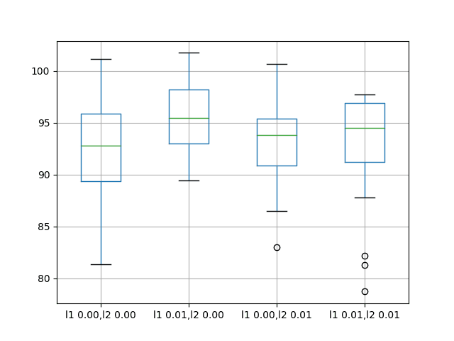
A box and whisker plot is also created to compare the distributions of results for each configuration.

The plot shows that all configurations have about the same spread and that the addition of bias regularization uniformly was not helpful on this problem.

Box and Whisker Plots of Bias Weight Regularization Performance on the Shampoo Sales Dataset

Input Weight Regularization

We can also apply regularization to input connections on each LSTM unit.

In Keras, this is achieved by setting the kernel_regularizer argument to a regularizer class.

We will test the same regularizer configurations as were used in the previous section, specifically:

L1L2(0.0, 0.0) [e.g. baseline]
L1L2(0.01, 0.0) [e.g. L1]
L1L2(0.0, 0.01) [e.g. L2]
L1L2(0.01, 0.01) [e.g. L1L2 or elasticnet]

Below lists the updated fit_lstm(), experiment(), and run() functions for using bias weight regularization with LSTMs.

# fit an LSTM network to training data
def fit_lstm(train, n_batch, nb_epoch, n_neurons, reg):
	X, y = train[:, 0:-1], train[:, -1]
	X = X.reshape(X.shape[0], 1, X.shape[1])
	model = Sequential()
	model.add(LSTM(n_neurons, batch_input_shape=(n_batch, X.shape[1], X.shape[2]), stateful=True, kernel_regularizer=reg))
	model.add(Dense(1))
	model.compile(loss='mean_squared_error', optimizer='adam')
	for i in range(nb_epoch):
		model.fit(X, y, epochs=1, batch_size=n_batch, verbose=0, shuffle=False)
		model.reset_states()
	return model

# run a repeated experiment
def experiment(series, n_lag, n_repeats, n_epochs, n_batch, n_neurons, reg):
	# transform data to be stationary
	raw_values = series.values
	diff_values = difference(raw_values, 1)
	# transform data to be supervised learning
	supervised = timeseries_to_supervised(diff_values, n_lag)
	supervised_values = supervised.values[n_lag:,:]
	# split data into train and test-sets
	train, test = supervised_values[0:-12], supervised_values[-12:]
	# transform the scale of the data
	scaler, train_scaled, test_scaled = scale(train, test)
	# run experiment
	error_scores = list()
	for r in range(n_repeats):
		# fit the model
		train_trimmed = train_scaled[2:, :]
		lstm_model = fit_lstm(train_trimmed, n_batch, n_epochs, n_neurons, reg)
		# forecast test dataset
		test_reshaped = test_scaled[:,0:-1]
		test_reshaped = test_reshaped.reshape(len(test_reshaped), 1, 1)
		output = lstm_model.predict(test_reshaped, batch_size=n_batch)
		predictions = list()
		for i in range(len(output)):
			yhat = output[i,0]
			X = test_scaled[i, 0:-1]
			# invert scaling
			yhat = invert_scale(scaler, X, yhat)
			# invert differencing
			yhat = inverse_difference(raw_values, yhat, len(test_scaled)+1-i)
			# store forecast
			predictions.append(yhat)
		# report performance
		rmse = sqrt(mean_squared_error(raw_values[-12:], predictions))
		print('%d) Test RMSE: %.3f' % (r+1, rmse))
		error_scores.append(rmse)
	return error_scores

# configure the experiment
def run():
	# load dataset
	series = read_csv('shampoo-sales.csv', header=0, parse_dates=[0], index_col=0, squeeze=True, date_parser=parser)
	# configure the experiment
	n_lag = 1
	n_repeats = 30
	n_epochs = 1000
	n_batch = 4
	n_neurons = 3
	regularizers = [L1L2(l1=0.0, l2=0.0), L1L2(l1=0.01, l2=0.0), L1L2(l1=0.0, l2=0.01), L1L2(l1=0.01, l2=0.01)]
	# run the experiment
	results = DataFrame()
	for reg in regularizers:
		name = ('l1 %.2f,l2 %.2f' % (reg.l1, reg.l2))
		results[name] = experiment(series, n_lag, n_repeats, n_epochs, n_batch, n_neurons, reg)
	# summarize results
	print(results.describe())
	# save boxplot
	results.boxplot()
	pyplot.savefig('experiment_reg_input.png')

# fit an LSTM network to training data

def fit_lstm(train, n_batch, nb_epoch, n_neurons, reg):

X, y = train[:, 0:-1], train[:, -1]

X = X.reshape(X.shape[0], 1, X.shape[1])

model = Sequential()

model.add(LSTM(n_neurons, batch_input_shape=(n_batch, X.shape[1], X.shape[2]), stateful=True, kernel_regularizer=reg))

model.add(Dense(1))

model.compile(loss='mean_squared_error', optimizer='adam')

for i in range(nb_epoch):

model.fit(X, y, epochs=1, batch_size=n_batch, verbose=0, shuffle=False)

model.reset_states()

return model

# run a repeated experiment

def experiment(series, n_lag, n_repeats, n_epochs, n_batch, n_neurons, reg):

# transform data to be stationary

raw_values = series.values

diff_values = difference(raw_values, 1)

# transform data to be supervised learning

supervised = timeseries_to_supervised(diff_values, n_lag)

supervised_values = supervised.values[n_lag:,:]

# split data into train and test-sets

train, test = supervised_values[0:-12], supervised_values[-12:]

# transform the scale of the data

scaler, train_scaled, test_scaled = scale(train, test)

# run experiment

error_scores = list()

for r in range(n_repeats):

# fit the model

train_trimmed = train_scaled[2:, :]

lstm_model = fit_lstm(train_trimmed, n_batch, n_epochs, n_neurons, reg)

# forecast test dataset

test_reshaped = test_scaled[:,0:-1]

test_reshaped = test_reshaped.reshape(len(test_reshaped), 1, 1)

output = lstm_model.predict(test_reshaped, batch_size=n_batch)

predictions = list()

for i in range(len(output)):

yhat = output[i,0]

X = test_scaled[i, 0:-1]

# invert scaling

yhat = invert_scale(scaler, X, yhat)

# invert differencing

yhat = inverse_difference(raw_values, yhat, len(test_scaled)+1-i)

# store forecast

predictions.append(yhat)

# report performance

rmse = sqrt(mean_squared_error(raw_values[-12:], predictions))

print('%d) Test RMSE: %.3f' % (r+1, rmse))

error_scores.append(rmse)

return error_scores

# configure the experiment

def run():

# load dataset

series = read_csv('shampoo-sales.csv', header=0, parse_dates=[0], index_col=0, squeeze=True, date_parser=parser)

# configure the experiment

n_lag = 1

n_repeats = 30

n_epochs = 1000

n_batch = 4

n_neurons = 3

regularizers = [L1L2(l1=0.0, l2=0.0), L1L2(l1=0.01, l2=0.0), L1L2(l1=0.0, l2=0.01), L1L2(l1=0.01, l2=0.01)]

# run the experiment

results = DataFrame()

for reg in regularizers:

name = ('l1 %.2f,l2 %.2f' % (reg.l1, reg.l2))

results[name] = experiment(series, n_lag, n_repeats, n_epochs, n_batch, n_neurons, reg)

# summarize results

print(results.describe())

# save boxplot

results.boxplot()

pyplot.savefig('experiment_reg_input.png')

Running this experiment prints descriptive statistics for each evaluated configuration.

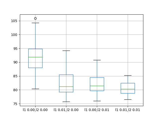
The results suggest that adding weight regularization to input connections does offer benefit across the board on this setup.

We can see that the test RMSE is approximately 10 units lower for all configurations with perhaps more benefit when both L1 and L2 are combined into an elasticnet type constraint.

       l1 0.00,l2 0.00  l1 0.01,l2 0.00  l1 0.00,l2 0.01  l1 0.01,l2 0.01
count        30.000000        30.000000        30.000000        30.000000
mean         91.640028        82.118980        82.137198        80.471685
std           6.086401         4.116072         3.378984         2.212213
min          80.392310        75.705210        76.005173        76.550909
25%          88.025135        79.237822        79.698162        78.780802
50%          91.843761        81.235433        81.463882        80.283913
75%          94.860117        85.510177        84.563980        82.443390
max         105.820586        94.210503        90.823454        85.243135

l1 0.00,l2 0.00 l1 0.01,l2 0.00 l1 0.00,l2 0.01 l1 0.01,l2 0.01

count 30.000000 30.000000 30.000000 30.000000

mean 91.640028 82.118980 82.137198 80.471685

std 6.086401 4.116072 3.378984 2.212213

min 80.392310 75.705210 76.005173 76.550909

25% 88.025135 79.237822 79.698162 78.780802

50% 91.843761 81.235433 81.463882 80.283913

75% 94.860117 85.510177 84.563980 82.443390

max 105.820586 94.210503 90.823454 85.243135

A box and whisker plot is also created to compare the distributions of results for each configuration.

The plot shows the general lower distribution of error for input regularization. The results also suggest a tighter spread of results with regularization that may be more pronounced with the L1L2 configuration that achieved the better results.

This is an encouraging finding, suggesting that additional experiments with different L1L2 values for input regularization would be well worth investigating.

Box and Whisker Plots of Input Weight Regularization Performance on the Shampoo Sales Dataset

Recurrent Weight Regularization

Finally, we can also apply regularization to recurrent connections on each LSTM unit.

In Keras, this is achieved by setting the recurrent_regularizer argument to a regularizer class.

We will test the same regularizer configurations as were used in the previous section, specifically:

L1L2(0.0, 0.0) [e.g. baseline]
L1L2(0.01, 0.0) [e.g. L1]
L1L2(0.0, 0.01) [e.g. L2]
L1L2(0.01, 0.01) [e.g. L1L2 or elasticnet]

Below lists the updated fit_lstm(), experiment(), and run() functions for using bias weight regularization with LSTMs.

# fit an LSTM network to training data
def fit_lstm(train, n_batch, nb_epoch, n_neurons, reg):
	X, y = train[:, 0:-1], train[:, -1]
	X = X.reshape(X.shape[0], 1, X.shape[1])
	model = Sequential()
	model.add(LSTM(n_neurons, batch_input_shape=(n_batch, X.shape[1], X.shape[2]), stateful=True, recurrent_regularizer=reg))
	model.add(Dense(1))
	model.compile(loss='mean_squared_error', optimizer='adam')
	for i in range(nb_epoch):
		model.fit(X, y, epochs=1, batch_size=n_batch, verbose=0, shuffle=False)
		model.reset_states()
	return model

# run a repeated experiment
def experiment(series, n_lag, n_repeats, n_epochs, n_batch, n_neurons, reg):
	# transform data to be stationary
	raw_values = series.values
	diff_values = difference(raw_values, 1)
	# transform data to be supervised learning
	supervised = timeseries_to_supervised(diff_values, n_lag)
	supervised_values = supervised.values[n_lag:,:]
	# split data into train and test-sets
	train, test = supervised_values[0:-12], supervised_values[-12:]
	# transform the scale of the data
	scaler, train_scaled, test_scaled = scale(train, test)
	# run experiment
	error_scores = list()
	for r in range(n_repeats):
		# fit the model
		train_trimmed = train_scaled[2:, :]
		lstm_model = fit_lstm(train_trimmed, n_batch, n_epochs, n_neurons, reg)
		# forecast test dataset
		test_reshaped = test_scaled[:,0:-1]
		test_reshaped = test_reshaped.reshape(len(test_reshaped), 1, 1)
		output = lstm_model.predict(test_reshaped, batch_size=n_batch)
		predictions = list()
		for i in range(len(output)):
			yhat = output[i,0]
			X = test_scaled[i, 0:-1]
			# invert scaling
			yhat = invert_scale(scaler, X, yhat)
			# invert differencing
			yhat = inverse_difference(raw_values, yhat, len(test_scaled)+1-i)
			# store forecast
			predictions.append(yhat)
		# report performance
		rmse = sqrt(mean_squared_error(raw_values[-12:], predictions))
		print('%d) Test RMSE: %.3f' % (r+1, rmse))
		error_scores.append(rmse)
	return error_scores

# configure the experiment
def run():
	# load dataset
	series = read_csv('shampoo-sales.csv', header=0, parse_dates=[0], index_col=0, squeeze=True, date_parser=parser)
	# configure the experiment
	n_lag = 1
	n_repeats = 30
	n_epochs = 1000
	n_batch = 4
	n_neurons = 3
	regularizers = [L1L2(l1=0.0, l2=0.0), L1L2(l1=0.01, l2=0.0), L1L2(l1=0.0, l2=0.01), L1L2(l1=0.01, l2=0.01)]
	# run the experiment
	results = DataFrame()
	for reg in regularizers:
		name = ('l1 %.2f,l2 %.2f' % (reg.l1, reg.l2))
		results[name] = experiment(series, n_lag, n_repeats, n_epochs, n_batch, n_neurons, reg)
	# summarize results
	print(results.describe())
	# save boxplot
	results.boxplot()
	pyplot.savefig('experiment_reg_recurrent.png')

# fit an LSTM network to training data

def fit_lstm(train, n_batch, nb_epoch, n_neurons, reg):

X, y = train[:, 0:-1], train[:, -1]

X = X.reshape(X.shape[0], 1, X.shape[1])

model = Sequential()

model.add(LSTM(n_neurons, batch_input_shape=(n_batch, X.shape[1], X.shape[2]), stateful=True, recurrent_regularizer=reg))

model.add(Dense(1))

model.compile(loss='mean_squared_error', optimizer='adam')

for i in range(nb_epoch):

model.fit(X, y, epochs=1, batch_size=n_batch, verbose=0, shuffle=False)

model.reset_states()

return model

# run a repeated experiment

def experiment(series, n_lag, n_repeats, n_epochs, n_batch, n_neurons, reg):

# transform data to be stationary

raw_values = series.values

diff_values = difference(raw_values, 1)

# transform data to be supervised learning

supervised = timeseries_to_supervised(diff_values, n_lag)

supervised_values = supervised.values[n_lag:,:]

# split data into train and test-sets

train, test = supervised_values[0:-12], supervised_values[-12:]

# transform the scale of the data

scaler, train_scaled, test_scaled = scale(train, test)

# run experiment

error_scores = list()

for r in range(n_repeats):

# fit the model

train_trimmed = train_scaled[2:, :]

lstm_model = fit_lstm(train_trimmed, n_batch, n_epochs, n_neurons, reg)

# forecast test dataset

test_reshaped = test_scaled[:,0:-1]

test_reshaped = test_reshaped.reshape(len(test_reshaped), 1, 1)

output = lstm_model.predict(test_reshaped, batch_size=n_batch)

predictions = list()

for i in range(len(output)):

yhat = output[i,0]

X = test_scaled[i, 0:-1]

# invert scaling

yhat = invert_scale(scaler, X, yhat)

# invert differencing

yhat = inverse_difference(raw_values, yhat, len(test_scaled)+1-i)

# store forecast

predictions.append(yhat)

# report performance

rmse = sqrt(mean_squared_error(raw_values[-12:], predictions))

print('%d) Test RMSE: %.3f' % (r+1, rmse))

error_scores.append(rmse)

return error_scores

# configure the experiment

def run():

# load dataset

series = read_csv('shampoo-sales.csv', header=0, parse_dates=[0], index_col=0, squeeze=True, date_parser=parser)

# configure the experiment

n_lag = 1

n_repeats = 30

n_epochs = 1000

n_batch = 4

n_neurons = 3

regularizers = [L1L2(l1=0.0, l2=0.0), L1L2(l1=0.01, l2=0.0), L1L2(l1=0.0, l2=0.01), L1L2(l1=0.01, l2=0.01)]

# run the experiment

results = DataFrame()

for reg in regularizers:

name = ('l1 %.2f,l2 %.2f' % (reg.l1, reg.l2))

results[name] = experiment(series, n_lag, n_repeats, n_epochs, n_batch, n_neurons, reg)

# summarize results

print(results.describe())

# save boxplot

results.boxplot()

pyplot.savefig('experiment_reg_recurrent.png')

Running this experiment prints descriptive statistics for each evaluated configuration.

The results suggest no obvious benefit from using regularization on the recurrent connection with LSTMs on this problem.

The mean performance of all variations tried resulted in worse performance than the baseline model.

       l1 0.00,l2 0.00  l1 0.01,l2 0.00  l1 0.00,l2 0.01  l1 0.01,l2 0.01
count        30.000000        30.000000        30.000000        30.000000
mean         92.918797       100.675386       101.302169        96.820026
std           7.172764         3.866547         5.228815         3.966710
min          72.967841        93.789854        91.063592        89.367600
25%          90.311185        98.014045        98.222732        94.787647
50%          92.327824       100.546756       101.903350        95.727549
75%          95.989761       103.491192       104.918266        98.240613
max         110.529422       108.788604       110.712064       111.185747

l1 0.00,l2 0.00 l1 0.01,l2 0.00 l1 0.00,l2 0.01 l1 0.01,l2 0.01

count 30.000000 30.000000 30.000000 30.000000

mean 92.918797 100.675386 101.302169 96.820026

std 7.172764 3.866547 5.228815 3.966710

min 72.967841 93.789854 91.063592 89.367600

25% 90.311185 98.014045 98.222732 94.787647

50% 92.327824 100.546756 101.903350 95.727549

75% 95.989761 103.491192 104.918266 98.240613

max 110.529422 108.788604 110.712064 111.185747

A box and whisker plot is also created to compare the distributions of results for each configuration.

The plot shows the same story as the summary statistics, suggesting little benefit from using recurrent weight regularization.

Box and Whisker Plots of Recurrent Weight Regularization Performance on the Shampoo Sales Dataset

Extensions

This section lists ideas for follow-up experiments to extend the work in this tutorial.

Input Weight Regularization. The experimental results for input weight regularization on this problem showed great promise of listing performance. This could be investigated further by perhaps grid searching different L1 and L2 values to find an optimal configuration.
Behavior Dynamics. The dynamic behavior of each weight regularization scheme could be investigated by plotting train and test RMSE over training epochs to get an idea of weight regularization on overfitting or underfitting behavior patterns.
Combine Regularization. Experiments could be designed to explore the effect of combining different weight regularization schemes.
Activation Regularization. Keras also supports activation regularization, and this could be another avenue to explore imposing constraints on the LSTM and reduce overfitting.

Summary

In this tutorial, you discovered how to use weight regularization with LSTMs for time series forecasting.

Specifically, you learned:

How to design a robust test harness for evaluating LSTM networks for time series forecasting.
How to configure bias weight regularization on LSTMs for time series forecasting.
How to configure input and recurrent weight regularization on LSTMs for time series forecasting.

Do you have any questions about using weight regularization with LSTM networks?
Ask your questions in the comments below and I will do my best to answer.

65 Responses to Weight Regularization with LSTM Networks for Time Series Forecasting

Alex May 5, 2017 at 5:57 am #

Gret job like every time.

But I want to understand why always we are using rmse and we don’t use the accuracy metrics ??

Reply
- Jason Brownlee May 5, 2017 at 7:35 am #
  
  You cannot measure accuracy on regression problems (unless you transform them to become a classification problem).
  
  In general, problems that have a real-valued quantity as the output variable are regression problems, those that have a category or label output are classification.
  
  Reply
Alex May 5, 2017 at 7:51 am #

Ah OK, yes it is a logic thinking. Thanks

Reply
shobhit May 5, 2017 at 9:08 pm #

hello jason,
how can be predicted a stock market data using a multiple input of columns and single output columns.

Reply
- Jason Brownlee May 6, 2017 at 7:42 am #
  
  Each separate time series would be framed as a separate feature in the LSTM.
  
  also, I believe short term security prices are a random walk and are not predictable:
  https://machinelearningmastery.com/gentle-introduction-random-walk-times-series-forecasting-python/
  
  Reply
shobhit May 5, 2017 at 9:18 pm #

import numpy as np
import pandas as pd
import tensorflow as tf
#tf.logging.set_verosity(tf.logging.ERROR)
from pandas_datareader import data as web
import matplotlib.pyplot as plt
def get_data():
feature_cols={‘ret_%s’ %i:tf.constant(idata[‘ret_%s’%i].values)for i in lags}
labels=tf.constant((idata[‘returns’]>0).astype(int).values,shape=[idata[‘returns’].size,1])
return feature_cols,labels

symbol=’^GSPC’
data=web.DataReader(symbol,data_source=’yahoo’,start=’2014-01-01′,end=’2016-10-31′)[‘Adj Close’]
data=pd.DataFrame(data)
data.rename(columns={‘Adj Close’:’price’},inplace=True)
data[‘returns’]=np.log(data/data.shift(1))
lags=range(1,6)
for i in lags:
data[‘ret_%s’% i]=np.sign(data[‘returns’].shift(i))
data.dropna(inplace=True)
print data.round(4).tail()
cutoff=’2015-1-1′
training_data=data[data.index=cutoff].copy()
#def get_data():
#feature_cols={‘ret_%s’ %i:tf.constant(data[‘ret_%s’%i].values)for i in lags}
#labels=tf.constant((data[‘returns’]>0).astype(int).values,shape=[data[‘returns’].size,1])
#return feature_cols,labels
fc=[tf.contrib.layers.real_valued_column(‘ret_%s’% i,dimension=1) for i in lags]
model=tf.contrib.learn.DNNClassifier(feature_columns=fc,n_classes=2,hidden_units=[100,100])
idata=training_data
model.fit(input_fn=get_data,steps=500)
model.evaluate(input_fn=get_data,steps=1)
pred=model.predict(input_fn=get_data)
pred[:30]
training_data[‘prediction’]=np.where(pred>0,1,-1)
training_data[‘strategy’]=training_data[‘prediction’]*training_data[‘returns’]
training_data[[‘returns’,’strategy’]].cumsum().apply(np.exp).plot(figsize=(10,6))
idata=test_data
model.evaluate(input_fn=get_data,steps=1)
pred=model.predict(input_fn=get_data)
test_data[‘prediction’]=np.where(pred>0,1,-1)
test_data[‘strategy’]=test_data[‘prediction’]*test_data[‘returns’]
test_data[[‘returns’,’strategy’]].cumsum().apply(np.exp).plot(figsize=(10,6))
#pred[:1]
if __name__ == ‘__main__’:
get_data()

hello jason,
i just ran this code but i got some error in the code and i cannot understand the error.
the error is:—–> 1 pred[:30]

TypeError: ‘generator’ object is not subscriptable

please kindly help me.

Reply
- Jason Brownlee May 6, 2017 at 7:43 am #
  
  Perhaps contact the author of the tensorflow code you have pasted?
  
  Reply
Birkey May 10, 2017 at 10:48 am #

Great article!
however, what confused me is, in section LSTM model, “A batch size of 1 is required as we will be using walk-forward validation and making one-step forecasts for each of the final 12 months of test data.”, but then you use batch size as 4 (n_batch=4).

I guess you mean “A time step of 1 is required”, am I right? cause one forecast per month means one time step.

Reply
- Jason Brownlee May 11, 2017 at 8:26 am #
  
  You make a good point.
  
  A batch size of 1 would be required if we made predictions each time step of the test data. Here we predict the whole year first, then work through the predictions to see what they mean.
  
  I have updated the post correcting the error.
  
  Reply
Laurent May 11, 2017 at 5:58 pm #

Thanks for all your pedagogic material, it’s really easy to learn with your articles!

I have a question: in all your examples of time series deep learning, you’re always predicting the next time step, one at a time.

How would you approach the case of training with a time series, and forecasting the next 12 steps, for example?

Reply
- Jason Brownlee May 12, 2017 at 7:37 am #
  
  Here is an example:
  https://machinelearningmastery.com/multi-step-time-series-forecasting-long-short-term-memory-networks-python/
  
  Reply
jinhua zhang May 12, 2017 at 4:31 am #

HI, your article is very useful for me! But I run the “Bias Weight Regularization procedure”, the spyder will have the fault :”D:\Program Files\Anaconda3\lib\site-packages\matplotlib\__init__.py:1357: UserWarning: This call to matplotlib.use() has no effect
because the backend has already been chosen;
matplotlib.use() must be called *before* pylab, matplotlib.pyplot,
or matplotlib.backends is imported for the first time.

warnings.warn(_use_error_msg)”,
I don’t know how to slove the fault, could you help me ?

Reply
- Jason Brownlee May 12, 2017 at 7:47 am #
  
  Are you able to run the script from the command line instead of within the IDE?
  
  Reply
  - jinhua zhang May 16, 2017 at 1:07 am #
    
    Thank you very much! Because I missed the command
    “# entry point
    run()”.
    When I added the command,the procedure could run.
    
    Reply
    - Jason Brownlee May 16, 2017 at 8:49 am #
      
      I’m glad to hear it.
      
      Reply
Neeraj Agrawal October 31, 2017 at 6:17 am #

I have one doubt related to stateful = True. As mentioned in keras documentation, first element of first batch is in sequence with first element of second batch and so on. But you have not converted time series into that order. Is it correct observation or I am missing something?

Reply
- conspiracypopcorn March 17, 2018 at 5:19 am #
  
  I’m pretty sure the implementation is wrong. If you check on the keras manual, the input to the LSTM should be (batch_size, timesteps, input_dim). The thing is that in this example we only have one sequence, so batch_size should be 1 and timesteps should be 4, not the opposite as shown in the article. Then it also makes sense that the state is kept between batches.
  
  Reply
SethM April 4, 2018 at 9:04 am #

I’m trying to understand how you’re attaching the regularizers to the model. In the fit_lstm(…) methods you’re never actually attaching anything in the reg variable to the model. Or, am I missing something? Thank you!

Reply
- Jason Brownlee April 5, 2018 at 5:46 am #
  
  They are specified on the LSTM layer via arguments.
  
  Reply
  - SethM April 8, 2018 at 2:15 am #
    
    Thank you! The code view widget was hiding it, my bad.
    
    Seth
    
    Reply
Rob May 5, 2018 at 2:14 pm #

Thanks for the post. Your posts are extremely valuable and I appreciate the time you are taking to write these.

Why did you choose the number of hidden layers in a LSTM as just 3? In general how does one decide to choose the number of hidden units?

Reply
- Jason Brownlee May 6, 2018 at 6:22 am #
  
  Great question. I used a little trial and error.
  
  For more on configuring neural nets, see this:
  https://machinelearningmastery.com/faq/single-faq/how-many-layers-and-nodes-do-i-need-in-my-neural-network
  
  Reply
Rob May 7, 2018 at 10:58 pm #

Thanks.

I am wondering if the number of hidden layers in LSTM is a function of the number of input samples to the model? ie each hidden layer has weights that needs to be learnt and if there is less data then there would be a tendency to overfit if we choose a large number of hidden layers.

On another note .. What is the dimension of the hidden layer ? For instance if the the input shape is (5,30) — (num of time steps, num of features) and the number of samples is 100,000 .. what would be the dimension of the first hidden layer and subsequent layers in LSTM

Regards,
-Avi

Reply
- Jason Brownlee May 8, 2018 at 6:13 am #
  
  No. Units in the first hidden layer has nothing to do with the length of input sequences.
  
  You can see the shape of each layer by printing the output of model.summary().
  
  Reply
Brian McDermott September 6, 2018 at 11:04 pm #

Hi Jason,

Thanks for sharing this article.

I have an LSTM network having 3 LSTM layers. I was wondering if I need to add recurrent regularization at each LSTM layer?

Reply
- Jason Brownlee September 7, 2018 at 8:04 am #
  
  Try it and see.
  
  Reply
Lee MH November 27, 2019 at 12:23 pm #

I’ve seen the good contents.

May I ask you a question personally? Can you emphasize specific variables in your predictions with LSTM?

When model calculate the weight of a variable, can you make a particular variable more important?

Reply
- Jason Brownlee November 27, 2019 at 1:51 pm #
  
  Thanks.
  
  No, the model will figure out what is most important during learning.
  
  Reply
Alok Singh January 24, 2020 at 1:26 am #

Hey thanks for nice explaination!!

My question is
Is there any difference in your bias weight regularization code and input weight regularization code because in both the way of use regularization is similar, how will the system identify that you want to use bias regularization or input weight regularization??

Reply
- Alok Singh January 24, 2020 at 1:27 am #
  
  Like for recurrent_regularizer you have specified it but what about input weight regularization
  
  Reply
- Alok Singh January 24, 2020 at 1:28 am #
  
  ohhh!! I got the answer
  
  Thanks man for the nice blog
  
  Reply
  - Jason Brownlee January 24, 2020 at 7:54 am #
    
    No problem.
    
    Reply
- Jason Brownlee January 24, 2020 at 7:54 am #
  
  Different arguments are used on the LSTM layers for bias vs weight regularization.
  
  Reply
Stephan February 17, 2020 at 2:18 pm #

Hello, Dr. Brownlee,
I have a question on validation:
What would be the best way to incorporate validation_split or validation_data parameter into the model.fit() with the setup you have outlined above? I.e. perform validation during training to asses over-fit.
validation_split does not seem to work…

Thanks

Reply
- Jason Brownlee February 18, 2020 at 6:15 am #
  
  Validation data for LSTMs is very tricky. You might be better off using walk-forward validation.
  
  Reply
AGGELOS PAPOUTSIS August 26, 2020 at 12:13 am #

hI,

Do you have any article about the inner procedures when we apply bias/weight or recurrent regularization? Thanks in advanced.

Reply
- AGGELOS PAPOUTSIS August 26, 2020 at 12:17 am #
  
  in other words which component is best to regularize?
  
  Reply
  - Jason Brownlee August 26, 2020 at 6:51 am #
    
    I recommend comparing the results from a suite of regularization techniques.
    
    Reply
- Jason Brownlee August 26, 2020 at 6:51 am #
  
  This might help as a starting point:
  https://machinelearningmastery.com/introduction-to-regularization-to-reduce-overfitting-and-improve-generalization-error/
  
  Reply
Jessy November 28, 2020 at 7:39 pm #

Extensions
This section lists ideas for follow-up experiments to extend the work in this tutorial.

Activation Regularization. Keras also supports activation regularization, and this could be another avenue to explore imposing constraints on the LSTM and reduce overfitting.

hi jason,
I read above work .in that you gave some extensions ….In particluar last work is activation regularization (activation function regularization ) is that correct . which means can i use regualrization techniques in the activation function in order to handle the overfitting concepts…way which i understood correct or wrong ..

Reply
- Jason Brownlee November 29, 2020 at 8:11 am #
  
  Yes, here is an example:
  https://machinelearningmastery.com/how-to-reduce-generalization-error-in-deep-neural-networks-with-activity-regularization-in-keras/
  
  Reply
Jessy January 20, 2021 at 10:59 am #

hi jason,
Can i use both weight regularization in LSTM and activation regularization in the HIDDEN LAYER at the same time in order to overcome the overfitting…

Reply
- Jason Brownlee January 20, 2021 at 12:41 pm #
  
  I don’t see why not, perhaps try it and compare results to not using it.
  
  Reply
  - Jessy January 21, 2021 at 12:36 pm #
    
    hi jason,
    is that possible to use lstm+ weight regularization +dropout techniques together to reduce overfitting….
    
    Reply
    - Jason Brownlee January 22, 2021 at 7:14 am #
      
      Yes, perhaps try the combination to see if it performs better on your dataset.
      
      Reply
Jessy January 22, 2021 at 12:03 pm #

hi jason,
is that possible to use activation regularization on LSTM Nodes in order to overcome overfitting

Reply
- Jason Brownlee January 22, 2021 at 1:23 pm #
  
  It can be used with LSTMs.
  
  It may or may not help with overfitting depending on the specifics of your model and dataset.
  
  Reply
Jessy January 28, 2021 at 2:56 pm #

hi jason ,
which regularization techniques L1(OR) L2 (OR) ELASTIC NET IS MORE SUITABLE ONE ON LSTM MODEL..

Reply
- Jason Brownlee January 29, 2021 at 5:59 am #
  
  It depends on the specifics of your model and dataset.
  
  Perhaps try a suite of approaches and discover what works best for you.
  
  Reply
Jessy January 28, 2021 at 7:04 pm #

hi jason,
using L1 regularization on lstm output layer and dropout in hidden (dense) layer to build a generalised model

Reply
- Jason Brownlee January 29, 2021 at 5:59 am #
  
  That sounds odd. Typically only one regularization method would be used in a model.
  
  Reply
Peter January 29, 2021 at 7:33 pm #

Hi Jason,

If you find that your deep model needs Batch Normalization, but still needs some regularization to prevent over fitting. What methods would apply to test?

I have read that Dropouts shouldn’t be used together with Batch Norm, also I have read that (at least some) methods of Lx regulation takes another role when combined with Batch Norm (https://blog.janestreet.com/l2-regularization-and-batch-norm/).

From your experience, what should I start experimenting with in a deep LSTM network with Batch Normalization, where I still experience over fitting?

Lets also assume that getting more data to train on is exhausted, and augmenting data is a very limited option.

Reply
- Jason Brownlee January 30, 2021 at 6:32 am #
  
  Dropout still works well, so does early stopping and weight decay.
  
  Also slow down learning with a smaller learning rate and more epochs.
  
  Generally, test a few methods and discover what works well/best for your model + data.
  
  Reply
Jessy February 16, 2021 at 9:56 pm #

hi jason,
does Lstm need feature extraction and feature selection of EEG signals… or automatically learn the required features from EEG signals

Reply
- Jason Brownlee February 17, 2021 at 5:27 am #
  
  It can learn to extract features from the signal.
  
  Reply
Jessy February 24, 2021 at 7:46 pm #

hi jason,
deep learning model (LSTM ) requires any explicit feature selection and feature extraction techniques when using EEG dataset

Reply
- Jason Brownlee February 25, 2021 at 5:27 am #
  
  It may or may not. Try with and without and compare the performance of the model on your dataset. Use what works best.
  
  Reply
Zainal October 6, 2021 at 6:20 pm #

Dear Prof. Jason Brownlee, thank you for this tutorial and explanation.
I want to ask, can we use this Weight Regularization-LSTM to classify something? for example, for HAR as also found on this website.
If so, are the steps the same?
I’m still just learning about LSTM and python, so sorry if my question is too basic.
Thank you very much.

Reply
- Adrian Tam October 7, 2021 at 2:58 am #
  
  Should work but LSTM is designed for time series so the network can remember something. Is that useful for classification? You can try out to confirm.
  
  Reply
José January 18, 2022 at 1:04 am #

Great article!!!.

Could you explain me why you use: X.reshape(X.shape[0], 1, X.shape[1])?

Thank you

Reply
- James Carmichael January 20, 2022 at 8:23 am #
  
  Hi Jose…Please see the following that relates to reshaping input data:
  
  https://machinelearningmastery.com/reshape-input-data-long-short-term-memory-networks-keras/
  
  Reply
Akkis August 21, 2022 at 7:34 pm #

hey!! can we modify the weight of LSTM using a function?
weight=f(x,y)
then, assigned it to model

Reply
- James Carmichael August 22, 2022 at 9:05 am #
  
  Hi Akkis…The following resource may be of interest:
  
  https://machinelearningmastery.com/update-lstm-networks-training-time-series-forecasting/
  
  Reply
Andrea October 17, 2022 at 7:49 pm #

How can one deduce which weights (and related to which inputs) have been regularized?

Reply
- James Carmichael October 18, 2022 at 10:02 am #
  
  Hi Andrea…The following resource may be of interest to you:
  
  https://machinelearningmastery.com/weight-regularization-to-reduce-overfitting-of-deep-learning-models/
  
  Reply

Navigation

Weight Regularization with LSTM Networks for Time Series Forecasting

Tutorial Overview

Environment

Need help with Deep Learning for Time Series?

Shampoo Sales Dataset

Experimental Test Harness

Data Split

Model Evaluation

Data Preparation

LSTM Model

Experimental Runs

Baseline LSTM Model

Bias Weight Regularization

Input Weight Regularization

Recurrent Weight Regularization

Extensions

Summary

Develop Deep Learning models for Time Series Today!

Develop Your Own Forecasting models in Minutes

Finally Bring Deep Learning to your Time Series Forecasting Projects

More On This Topic

65 Responses to Weight Regularization with LSTM Networks for Time Series Forecasting

Leave a Reply Click here to cancel reply.