Understand the Impact of Learning Rate on Neural Network Performance

Deep learning neural networks are trained using the stochastic gradient descent optimization algorithm.

The learning rate is a hyperparameter that controls how much to change the model in response to the estimated error each time the model weights are updated. Choosing the learning rate is challenging as a value too small may result in a long training process that could get stuck, whereas a value too large may result in learning a sub-optimal set of weights too fast or an unstable training process.

The learning rate may be the most important hyperparameter when configuring your neural network. Therefore it is vital to know how to investigate the effects of the learning rate on model performance and to build an intuition about the dynamics of the learning rate on model behavior.

In this tutorial, you will discover the effects of the learning rate, learning rate schedules, and adaptive learning rates on model performance.

After completing this tutorial, you will know:

• How large learning rates result in unstable training and tiny rates result in a failure to train.
• Momentum can accelerate training and learning rate schedules can help to converge the optimization process.
• Adaptive learning rates can accelerate training and alleviate some of the pressure of choosing a learning rate and learning rate schedule.

Kick-start your project with my new book Better Deep Learning, including step-by-step tutorials and the Python source code files for all examples.

Let’s get started.

• Updated Feb/2019: Fixed issue where callbacks were mistakenly defined on compile() instead of fit() functions.
• Updated Oct/2019: Updated for Keras 2.3 and TensorFlow 2.0.
• Update Jan/2020: Updated for changes in scikit-learn v0.22 API.

Understand the Dynamics of Learning Rate on Model Performance With Deep Learning Neural Networks
Photo by Abdul Rahman some rights reserved

Tutorial Overview

This tutorial is divided into six parts; they are:

1. Learning Rate and Gradient Descent
2. Configure the Learning Rate in Keras
3. Multi-Class Classification Problem
4. Effect of Learning Rate and Momentum
5. Effect of Learning Rate Schedules
6. Effect of Adaptive Learning Rates

Learning Rate and Gradient Descent

Deep learning neural networks are trained using the stochastic gradient descent algorithm.

Stochastic gradient descent is an optimization algorithm that estimates the error gradient for the current state of the model using examples from the training dataset, then updates the weights of the model using the back-propagation of errors algorithm, referred to as simply backpropagation.

The amount that the weights are updated during training is referred to as the step size or the “learning rate.”

Specifically, the learning rate is a configurable hyperparameter used in the training of neural networks that has a small positive value, often in the range between 0.0 and 1.0.

The learning rate controls how quickly the model is adapted to the problem. Smaller learning rates require more training epochs given the smaller changes made to the weights each update, whereas larger learning rates result in rapid changes and require fewer training epochs.

A learning rate that is too large can cause the model to converge too quickly to a suboptimal solution, whereas a learning rate that is too small can cause the process to get stuck.

The challenge of training deep learning neural networks involves carefully selecting the learning rate. It may be the most important hyperparameter for the model.

The learning rate is perhaps the most important hyperparameter. If you have time to tune only one hyperparameter, tune the learning rate.

— Page 429, Deep Learning, 2016.

Now that we are familiar with what the learning rate is, let’s look at how we can configure the learning rate for neural networks.

For more on what the learning rate is and how it works, see the post:

• How to Configure the Learning Rate Hyperparameter When Training Deep Learning Neural Networks

Configure the Learning Rate in Keras

The Keras deep learning library allows you to easily configure the learning rate for a number of different variations of the stochastic gradient descent optimization algorithm.

Stochastic Gradient Descent

Keras provides the SGD class that implements the stochastic gradient descent optimizer with a learning rate and momentum.

First, an instance of the class must be created and configured, then specified to the “optimizer” argument when calling the fit() function on the model.

The default learning rate is 0.01 and no momentum is used by default.

The learning rate can be specified via the “lr” argument and the momentum can be specified via the “momentum” argument.

The class also supports learning rate decay via the “decay” argument.

With learning rate decay, the learning rate is calculated each update (e.g. end of each mini-batch) as follows:

Where lrate is the learning rate for the current epoch, initial_lrate is the learning rate specified as an argument to SGD, decay is the decay rate which is greater than zero and iteration is the current update number.

Learning Rate Schedule

Keras supports learning rate schedules via callbacks.

The callbacks operate separately from the optimization algorithm, although they adjust the learning rate used by the optimization algorithm. It is recommended to use the SGD when using a learning rate schedule callback.

Callbacks are instantiated and configured, then specified in a list to the “callbacks” argument of the fit() function when training the model.

Keras provides the ReduceLROnPlateau that will adjust the learning rate when a plateau in model performance is detected, e.g. no change for a given number of training epochs. This callback is designed to reduce the learning rate after the model stops improving with the hope of fine-tuning model weights.

The ReduceLROnPlateau requires you to specify the metric to monitor during training via the “monitor” argument, the value that the learning rate will be multiplied by via the “factor” argument and the “patience” argument that specifies the number of training epochs to wait before triggering the change in learning rate.

For example, we can monitor the validation loss and reduce the learning rate by an order of magnitude if validation loss does not improve for 100 epochs:

Keras also provides LearningRateScheduler callback that allows you to specify a function that is called each epoch in order to adjust the learning rate.

You can define your Python function that takes two arguments (epoch and current learning rate) and returns the new learning rate.

Adaptive Learning Rate Gradient Descent

Keras also provides a suite of extensions of simple stochastic gradient descent that support adaptive learning rates.

Because each method adapts the learning rate, often one learning rate per model weight, little configuration is often required.

Three commonly used adaptive learning rate methods include:

RMSProp Optimizer

Adagrad Optimizer

Adam Optimizer

Multi-Class Classification Problem

We will use a small multi-class classification problem as the basis to demonstrate the effect of learning rate on model performance.

The scikit-learn class provides the make_blobs() function that can be used to create a multi-class classification problem with the prescribed number of samples, input variables, classes, and variance of samples within a class.

The problem has two input variables (to represent the x and y coordinates of the points) and a standard deviation of 2.0 for points within each group. We will use the same random state (seed for the pseudorandom number generator) to ensure that we always get the same data points.

The results are the input and output elements of a dataset that we can model.

In order to get a feeling for the complexity of the problem, we can plot each point on a two-dimensional scatter plot and color each point by class value.

The complete example is listed below.

Running the example creates a scatter plot of the entire dataset. We can see that the standard deviation of 2.0 means that the classes are not linearly separable (separable by a line), causing many ambiguous points.

This is desirable as it means that the problem is non-trivial and will allow a neural network model to find many different “good enough” candidate solutions.

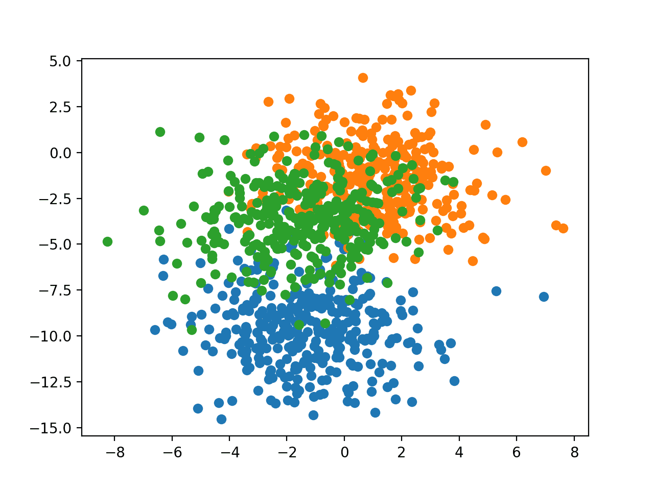
Scatter Plot of Blobs Dataset With Three Classes and Points Colored by Class Value

Effect of Learning Rate and Momentum

In this section, we will develop a Multilayer Perceptron (MLP) model to address the blobs classification problem and investigate the effect of different learning rates and momentum.

Learning Rate Dynamics

The first step is to develop a function that will create the samples from the problem and split them into train and test datasets.

Additionally, we must also one hot encode the target variable so that we can develop a model that predicts the probability of an example belonging to each class.

The prepare_data() function below implements this behavior, returning train and test sets split into input and output elements.

Next, we can develop a function to fit and evaluate an MLP model.

First, we will define a simple MLP model that expects two input variables from the blobs problem, has a single hidden layer with 50 nodes, and an output layer with three nodes to predict the probability for each of the three classes. Nodes in the hidden layer will use the rectified linear activation function (ReLU), whereas nodes in the output layer will use the softmax activation function.

We will use the stochastic gradient descent optimizer and require that the learning rate be specified so that we can evaluate different rates. The model will be trained to minimize cross entropy.

The model will be fit for 200 training epochs, found with a little trial and error, and the test set will be used as the validation dataset so we can get an idea of the generalization error of the model during training.

Once fit, we will plot the accuracy of the model on the train and test sets over the training epochs.

The fit_model() function below ties together these elements and will fit a model and plot its performance given the train and test datasets as well as a specific learning rate to evaluate.

We can now investigate the dynamics of different learning rates on the train and test accuracy of the model.

In this example, we will evaluate learning rates on a logarithmic scale from 1E-0 (1.0) to 1E-7 and create line plots for each learning rate by calling the fit_model() function.

Tying all of this together, the complete example is listed below.

Running the example creates a single figure that contains eight line plots for the eight different evaluated learning rates. Classification accuracy on the training dataset is marked in blue, whereas accuracy on the test dataset is marked in orange.

Note: Your results may vary given the stochastic nature of the algorithm or evaluation procedure, or differences in numerical precision. Consider running the example a few times and compare the average outcome.

The plots show oscillations in behavior for the too-large learning rate of 1.0 and the inability of the model to learn anything with the too-small learning rates of 1E-6 and 1E-7.

We can see that the model was able to learn the problem well with the learning rates 1E-1, 1E-2 and 1E-3, although successively slower as the learning rate was decreased. With the chosen model configuration, the results suggest a moderate learning rate of 0.1 results in good model performance on the train and test sets.

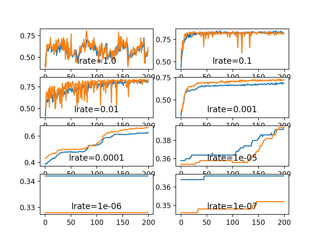
Line Plots of Train and Test Accuracy for a Suite of Learning Rates on the Blobs Classification Problem

Momentum Dynamics

Momentum can smooth the progression of the learning algorithm that, in turn, can accelerate the training process.

We can adapt the example from the previous section to evaluate the effect of momentum with a fixed learning rate. In this case, we will choose the learning rate of 0.01 that in the previous section converged to a reasonable solution, but required more epochs than the learning rate of 0.1

The fit_model() function can be updated to take a “momentum” argument instead of a learning rate argument, that can be used in the configuration of the SGD class and reported on the resulting plot.

The updated version of this function is listed below.

It is common to use momentum values close to 1.0, such as 0.9 and 0.99.

In this example, we will demonstrate the dynamics of the model without momentum compared to the model with momentum values of 0.5 and the higher momentum values.

Tying all of this together, the complete example is listed below.

Running the example creates a single figure that contains four line plots for the different evaluated momentum values. Classification accuracy on the training dataset is marked in blue, whereas accuracy on the test dataset is marked in orange.

Note: Your results may vary given the stochastic nature of the algorithm or evaluation procedure, or differences in numerical precision. Consider running the example a few times and compare the average outcome.

We can see that the addition of momentum does accelerate the training of the model. Specifically, momentum values of 0.9 and 0.99 achieve reasonable train and test accuracy within about 50 training epochs as opposed to 200 training epochs when momentum is not used.

In all cases where momentum is used, the accuracy of the model on the holdout test dataset appears to be more stable, showing less volatility over the training epochs.

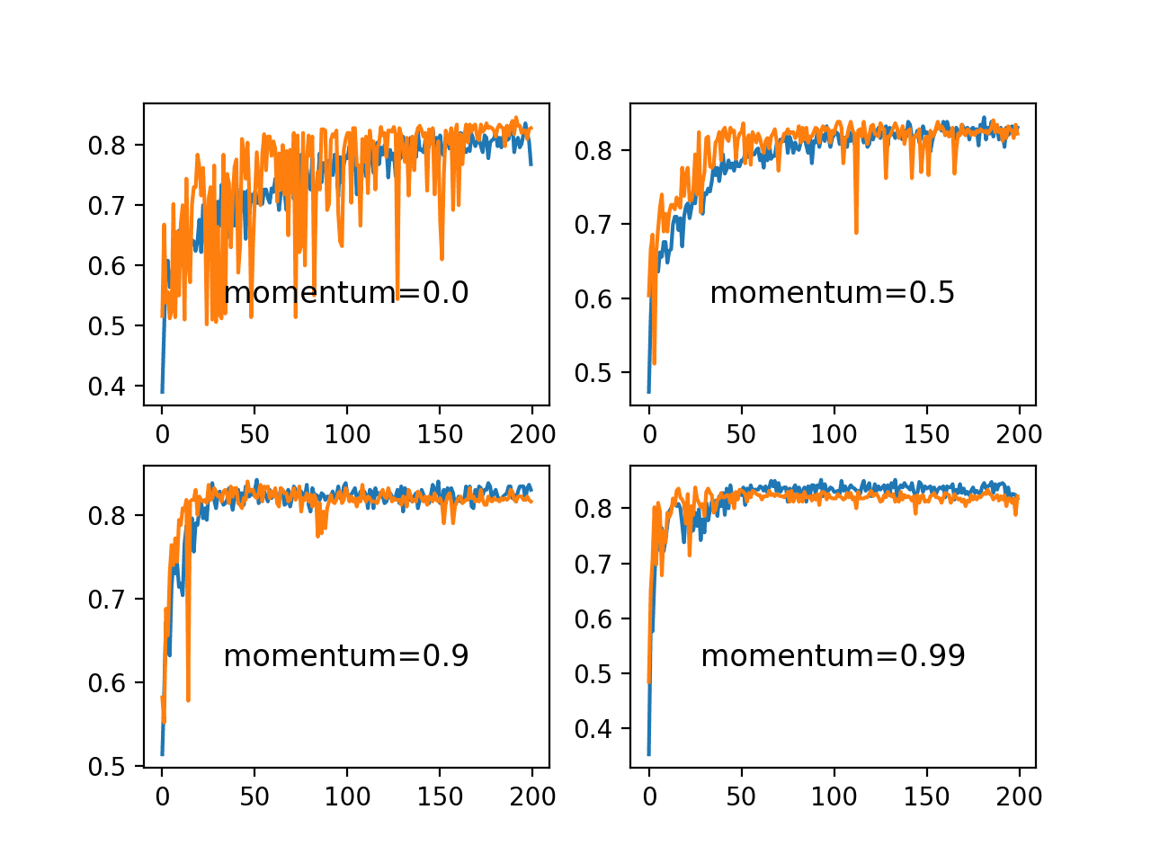
Line Plots of Train and Test Accuracy for a Suite of Momentums on the Blobs Classification Problem

Effect of Learning Rate Schedules

We will look at two learning rate schedules in this section.

The first is the decay built into the SGD class and the second is the ReduceLROnPlateau callback.

Learning Rate Decay

The SGD class provides the “decay” argument that specifies the learning rate decay.

It may not be clear from the equation or the code as to the effect that this decay has on the learning rate over updates. We can make this clearer with a worked example.

The function below implements the learning rate decay as implemented in the SGD class.

We can use this function to calculate the learning rate over multiple updates with different decay values.

We will compare a range of decay values [1E-1, 1E-2, 1E-3, 1E-4] with an initial learning rate of 0.01 and 200 weight updates.

The complete example is listed below.

Running the example creates a line plot showing learning rates over updates for different decay values.

We can see that in all cases, the learning rate starts at the initial value of 0.01. We can see that a small decay value of 1E-4 (red) has almost no effect, whereas a large decay value of 1E-1 (blue) has a dramatic effect, reducing the learning rate to below 0.002 within 50 epochs (about one order of magnitude less than the initial value) and arriving at the final value of about 0.0004 (about two orders of magnitude less than the initial value).

We can see that the change to the learning rate is not linear. We can also see that changes to the learning rate are dependent on the batch size, after which an update is performed. In the example from the previous section, a default batch size of 32 across 500 examples results in 16 updates per epoch and 3,200 updates across the 200 epochs.

Using a decay of 0.1 and an initial learning rate of 0.01, we can calculate the final learning rate to be a tiny value of about 3.1E-05.

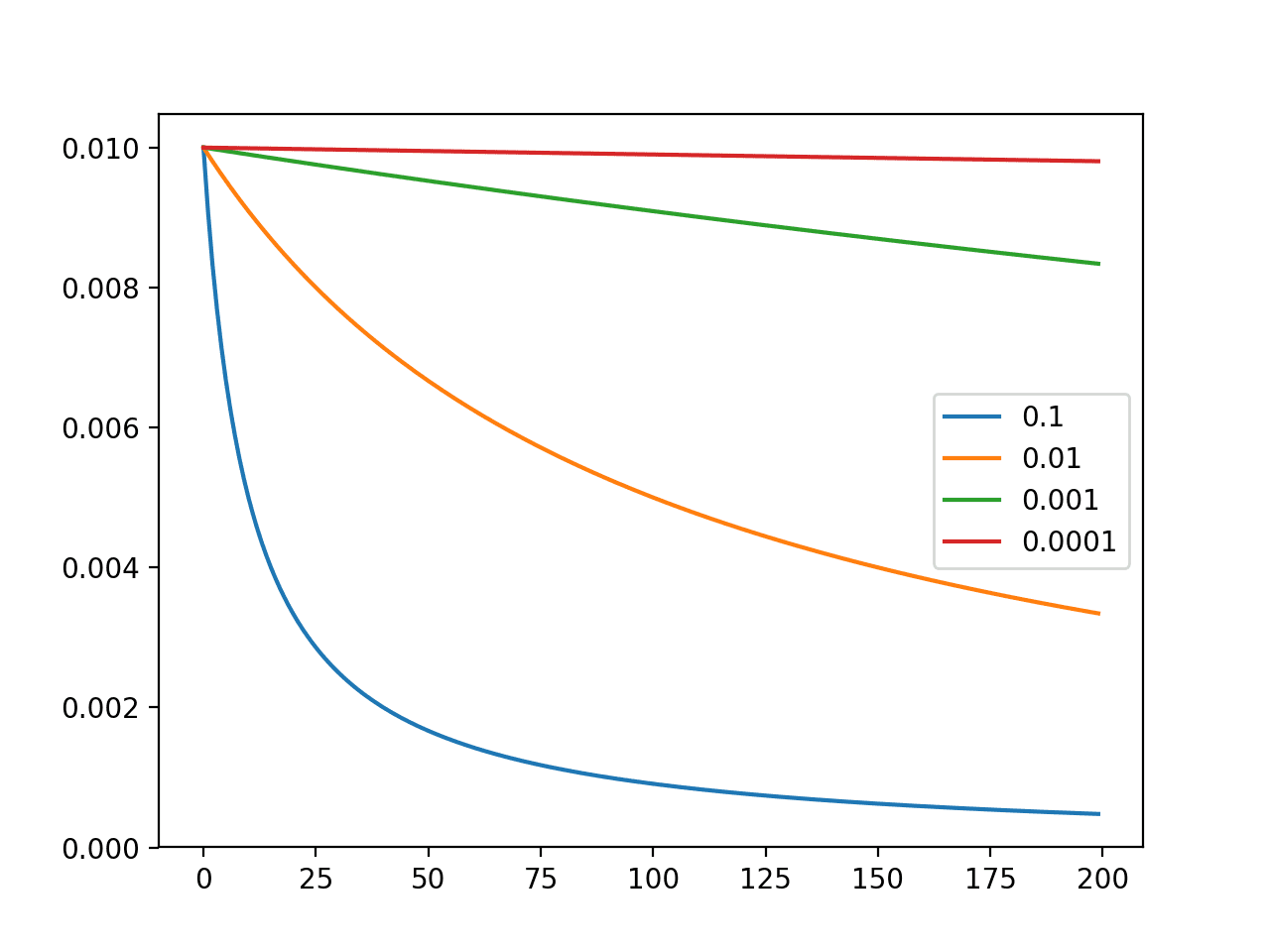
Line Plot of the Effect of Decay on Learning Rate Over Multiple Weight Updates

We can update the example from the previous section to evaluate the dynamics of different learning rate decay values.

Fixing the learning rate at 0.01 and not using momentum, we would expect that a very small learning rate decay would be preferred, as a large learning rate decay would rapidly result in a learning rate that is too small for the model to learn effectively.

The fit_model() function can be updated to take a “decay” argument that can be used to configure decay for the SGD class.

The updated version of the function is listed below.

We can evaluate the same four decay values of [1E-1, 1E-2, 1E-3, 1E-4] and their effect on model accuracy.

The complete example is listed below.

Running the example creates a single figure that contains four line plots for the different evaluated learning rate decay values. Classification accuracy on the training dataset is marked in blue, whereas accuracy on the test dataset is marked in orange.

Note: Your results may vary given the stochastic nature of the algorithm or evaluation procedure, or differences in numerical precision. Consider running the example a few times and compare the average outcome.

We can see that the large decay values of 1E-1 and 1E-2 indeed decay the learning rate too rapidly for this model on this problem and result in poor performance. The smaller decay values do result in better performance, with the value of 1E-4 perhaps causing in a similar result as not using decay at all. In fact, we can calculate the final learning rate with a decay of 1E-4 to be about 0.0075, only a little bit smaller than the initial value of 0.01.

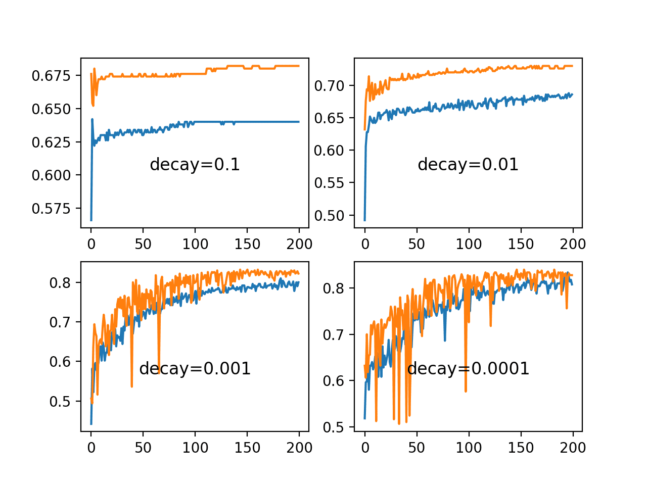
Line Plots of Train and Test Accuracy for a Suite of Decay Rates on the Blobs Classification Problem

Drop Learning Rate on Plateau

The ReduceLROnPlateau will drop the learning rate by a factor after no change in a monitored metric for a given number of epochs.

We can explore the effect of different “patience” values, which is the number of epochs to wait for a change before dropping the learning rate. We will use the default learning rate of 0.01 and drop the learning rate by an order of magnitude by setting the “factor” argument to 0.1.

It will be interesting to review the effect on the learning rate over the training epochs. We can do that by creating a new Keras Callback that is responsible for recording the learning rate at the end of each training epoch. We can then retrieve the recorded learning rates and create a line plot to see how the learning rate was affected by drops.

We can create a custom Callback called LearningRateMonitor. The on_train_begin() function is called at the start of training, and in it we can define an empty list of learning rates. The on_epoch_end() function is called at the end of each training epoch and in it we can retrieve the optimizer and the current learning rate from the optimizer and store it in the list. The complete LearningRateMonitor callback is listed below.

The fit_model() function developed in the previous sections can be updated to create and configure the ReduceLROnPlateau callback and our new LearningRateMonitor callback and register them with the model in the call to fit.

The function will also take “patience” as an argument so that we can evaluate different values.

We will want to create a few plots in this example, so instead of creating subplots directly, the fit_model() function will return the list of learning rates as well as loss and accuracy on the training dataset for each training epochs.

The function with these updates is listed below.

The patience in the ReduceLROnPlateau controls how often the learning rate will be dropped.

We will test a few different patience values suited for this model on the blobs problem and keep track of the learning rate, loss, and accuracy series from each run.

At the end of the run, we will create figures with line plots for each of the patience values for the learning rates, training loss, and training accuracy for each patience value.

We can create a helper function to easily create a figure with subplots for each series that we have recorded.

Tying these elements together, the complete example is listed below.

Running the example creates three figures, each containing a line plot for the different patience values.

Note: Your results may vary given the stochastic nature of the algorithm or evaluation procedure, or differences in numerical precision. Consider running the example a few times and compare the average outcome.

The first figure shows line plots of the learning rate over the training epochs for each of the evaluated patience values. We can see that the smallest patience value of two rapidly drops the learning rate to a minimum value within 25 epochs, the largest patience of 15 only suffers one drop in the learning rate.

From these plots, we would expect the patience values of 5 and 10 for this model on this problem to result in better performance as they allow the larger learning rate to be used for some time before dropping the rate to refine the weights.

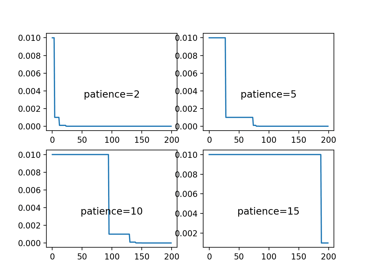
Line Plots of Learning Rate Over Epochs for Different Patience Values Used in the ReduceLROnPlateau Schedule

The next figure shows the loss on the training dataset for each of the patience values.

The plot shows that the patience values of 2 and 5 result in a rapid convergence of the model, perhaps to a sub-optimal loss value. In the case of a patience level of 10 and 15, loss drops reasonably until the learning rate is dropped below a level that large changes to the loss can be seen. This occurs halfway for the patience of 10 and nearly the end of the run for patience 15.

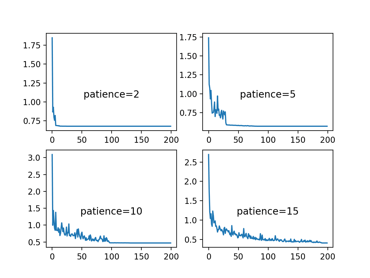
Line Plots of Training Loss Over Epochs for Different Patience Values Used in the ReduceLROnPlateau Schedule

The final figure shows the training set accuracy over training epochs for each patience value.

We can see that indeed the small patience values of 2 and 5 epochs results in premature convergence of the model to a less-than-optimal model at around 65% and less than 75% accuracy respectively. The larger patience values result in better performing models, with the patience of 10 showing convergence just before 150 epochs, whereas the patience 15 continues to show the effects of a volatile accuracy given the nearly completely unchanged learning rate.

These plots show how a learning rate that is decreased a sensible way for the problem and chosen model configuration can result in both a skillful and converged stable set of final weights, a desirable property in a final model at the end of a training run.

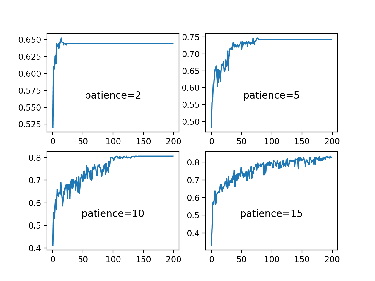
Line Plots of Training Accuracy Over Epochs for Different Patience Values Used in the ReduceLROnPlateau Schedule

Effect of Adaptive Learning Rates

Learning rates and learning rate schedules are both challenging to configure and critical to the performance of a deep learning neural network model.

Keras provides a number of different popular variations of stochastic gradient descent with adaptive learning rates, such as:

• Adaptive Gradient Algorithm (AdaGrad).
• Root Mean Square Propagation (RMSprop).
• Adaptive Moment Estimation (Adam).

Each provides a different methodology for adapting learning rates for each weight in the network.

There is no single best algorithm, and the results of racing optimization algorithms on one problem are unlikely to be transferable to new problems.

We can study the dynamics of different adaptive learning rate methods on the blobs problem. The fit_model() function can be updated to take the name of an optimization algorithm to evaluate, which can be specified to the “optimizer” argument when the MLP model is compiled. The default parameters for each method will then be used. The updated version of the function is listed below.

We can explore the three popular methods of RMSprop, AdaGrad and Adam and compare their behavior to simple stochastic gradient descent with a static learning rate.

We would expect the adaptive learning rate versions of the algorithm to perform similarly or better, perhaps adapting to the problem in fewer training epochs, but importantly, to result in a more stable model.

Tying these elements together, the complete example is listed below.

Running the example creates a single figure that contains four line plots for the different evaluated optimization algorithms. Classification accuracy on the training dataset is marked in blue, whereas accuracy on the test dataset is marked in orange.

Note: Your results may vary given the stochastic nature of the algorithm or evaluation procedure, or differences in numerical precision. Consider running the example a few times and compare the average outcome.

Again, we can see that SGD with a default learning rate of 0.01 and no momentum does learn the problem, but requires nearly all 200 epochs and results in volatile accuracy on the training data and much more so on the test dataset. The plots show that all three adaptive learning rate methods learning the problem faster and with dramatically less volatility in train and test set accuracy.

Both RMSProp and Adam demonstrate similar performance, effectively learning the problem within 50 training epochs and spending the remaining training time making very minor weight updates, but not converging as we saw with the learning rate schedules in the previous section.

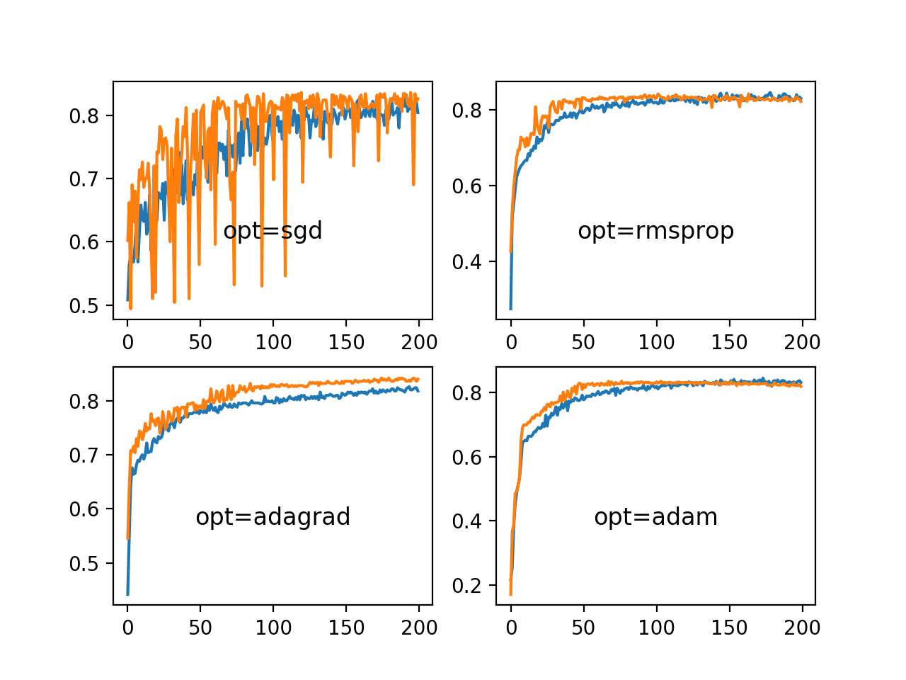
Line Plots of Train and Test Accuracy for a Suite of Adaptive Learning Rate Methods on the Blobs Classification Problem

Further Reading

This section provides more resources on the topic if you are looking to go deeper.

Posts

• How to Configure the Learning Rate Hyperparameter When Training Deep Learning Neural Networks

Papers

• Practical recommendations for gradient-based training of deep architectures, 2012.

Books

• Chapter 8: Optimization for Training Deep Models, Deep Learning, 2016.
• Chapter 6: Learning Rate and Momentum, Neural Smithing: Supervised Learning in Feedforward Artificial Neural Networks, 1999.
• Section 5.7: Gradient descent, Neural Networks for Pattern Recognition, 1995.

API

• Keras Optimizers API
• Keras Callbacks API
• optimizers.py Keras Source Code

Articles

• Stochastic gradient descent, Wikipedia.
• What learning rate should be used for backprop?, Neural Network FAQ.

Summary

In this tutorial, you discovered the effects of the learning rate, learning rate schedules, and adaptive learning rates on model performance.

Specifically, you learned:

• How large learning rates result in unstable training and tiny rates result in a failure to train.
• Momentum can accelerate training and learning rate schedules can help to converge the optimization process.
• Adaptive learning rates can accelerate training and alleviate some of the pressure of choosing a learning rate and learning rate schedule.

Do you have any questions?
Ask your questions in the comments below and I will do my best to answer.

Develop Better Deep Learning Models Today!

Train Faster, Reduce Overftting, and Ensembles

...with just a few lines of python code

Discover how in my new Ebook:
Better Deep Learning

It provides self-study tutorials on topics like:
weight decay, batch normalization, dropout, model stacking and much more...

Bring better deep learning to your projects!

Skip the Academics. Just Results.

See What's Inside