Indoor Movement Time Series Classification with Machine Learning Algorithms

Indoor movement prediction involves using wireless sensor strength data to predict the location and motion of subjects within a building.

It is a challenging problem as there is no direct analytical model to translate the variable length traces of signal strength data from multiple sensors into user behavior.

The ‘indoor user movement‘ dataset is a standard and freely available time series classification problem.

In this tutorial, you will discover the indoor movement prediction time series classification problem and how to engineer features and evaluate machine learning algorithms for the problem.

After completing this tutorial, you will know:

• The time series classification problem of predicting the movement between rooms based on sensor strength.
• How to investigate the data in order to better understand the problem and how to engineer features from the raw data for predictive modeling.
• How to spot check a suite of classification algorithms and tune one algorithm to further lift performance on the problem.

Kick-start your project with my new book Deep Learning for Time Series Forecasting, including step-by-step tutorials and the Python source code files for all examples.

Let’s get started.

• Update Sept/2018: Added a link to a mirror of the dataset.

Indoor Movement Time Series Classification with Machine Learning Algorithms
Photo by Nola Tularosa, some rights reserved.

Tutorial Overview

This tutorial is divided into five parts; they are:

1. Indoor User Movement Prediction
2. Indoor Movement Prediction Dataset
3. Model Evaluation
4. Data Preparation
5. Algorithm Spot-Check

Indoor User Movement Prediction

The ‘indoor user movement‘ prediction problem involves determining whether an individual has moved between rooms based on the change in signal strength measured by wireless detectors in the environment.

The dataset was collected and made available by Davide Bacciu, et al. from the University of Pisa in Italy and first described in their 2011 paper “Predicting User Movements in Heterogeneous Indoor Environments by Reservoir Computing” as a dataset for exploring a methodology that seems like recurrent neural networks called ‘reservoir computing.’

The problem is a special case of the more generic problem of predicting indoor user localization and movement patterns.

Data was collected by positioning four wireless sensors in the environment and one on the subject. The subject moved through the environment while the four wireless sensors detected and recorded a time series of sensor strength.

The result is a dataset comprised of variable length time series with four variates describing trajectory through a well-defined static environment, and the classification of whether the movement led to the subject changing rooms in the environment.

It is a challenging problem because there is no obvious and generic way to relate signal strength data to subject location in an environment.

The relationship between the RSS and the location of the tracked object cannot be easily formulated into an analytical model, as it strongly depends on the characteristics of the environment as well as on the wireless devices involved. I

— Predicting User Movements in Heterogeneous Indoor Environments by Reservoir Computing, 2011.

The data was collected under controlled experimental conditions.

Sensors were placed in three pairs of two connected rooms containing typical office furniture. Two sensors were placed in the corners of each of the two rooms and the subject walked one of six predefined paths through the rooms. Predictions are made at a point along each path that may or may not lead to a change of room.

The cartoon below makes this clear, showing the sensor locations (A1-A4), the six possible paths that may be walked, and the two points (M) where a prediction will be made.

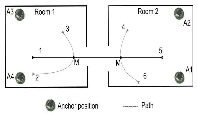
Overview of two rooms, sensor locations and the 6 pre-defined paths.
Taken from “Predicting User Movements in Heterogeneous Indoor Environments by Reservoir Computing.”

Three datasets were collected from the three pairs of two rooms in which the paths were walked and sensor measurements taken, referred to as Dataset 1, Dataset 2, and Dataset 3.

The table below, taken from the paper, summarizes the number of paths walked in each of the three datasets, the total number of room changes and non-room-changes (class label), and the lengths of the time series inputs.

Summary of sensor data collected from the three pairs of two rooms.
Taken from “Predicting User Movements in Heterogeneous Indoor Environments by Reservoir Computing.”

Technically, the data is comprised of multivariate time series inputs and a classification output and may be described as a time series classification problem.

The RSS values from the four anchors are organized into sequences of varying length corresponding to trajectory measurements from the starting point until marker M. A target classification label is associated to each input sequence to indicate whether the user is about to change its location (room) or not.

— Predicting User Movements in Heterogeneous Indoor Environments by Reservoir Computing, 2011.

Indoor Movement Prediction Dataset

The dataset is freely available from the UCI Machine Learning Repository:

• Indoor User Movement Prediction from RSS data Data Set, UCI Machine Learning Repository

In case the above site goes down (which can happen), here is a direct link to a mirror of the dataset:

• IndoorMovement.zip

The data can be downloaded as a .zip file that contains the following salient files:

• dataset/MovementAAL_RSS_???.csv The RSS traces for each movement, where ‘???’ in the filename marks the trace number from 1 to 311.
• dataset/MovementAAL_target.csv The mapping of trace number to the output class value or target.
• groups/MovementAAL_DatasetGroup.csv The mapping of trace number to the dataset group 1, 2, or 3 marking the pair of rooms from which the trace was recorded.
• groups/MovementAAL_Paths.csv The mapping of trace number to the path type, 1-6, marked in the cartoon diagram above.

The provided data is already normalized.

Specifically, each input variable is normalized into the range [-1,1] per dataset (pair of rooms), and the output class variable is marked -1 for no transition between rooms and +1 for a transition through the rooms.

[…] put data comprises time series of 4 dimensional RSS measurements (NU = 4) corresponding to the 4 anchors […] normalized in the range [−1, 1] independently for each dataset

— Predicting User Movements in Heterogeneous Indoor Environments by Reservoir Computing, 2011.

The scaling of data by dataset may (or may not) introduce additional challenges when combining observations across datasets if the pre-normalized distributions differ greatly.

The time series for one trace in a given trace file are provided in temporal order, where one row records the observations for a single time step. The data is recorded at 8Hz, meaning that one second of clock time elapses for eight time steps in the data.

Below is an example of a trace, taken from ‘dataset/MovementAAL_RSS_1.csv‘, which has the output target ‘1’ (a room transition occurred), from group 1 (the first pair of rooms) and is the path 1 (a straight shot from left to right between the rooms).

The datasets were used in two specific ways (experimental settings or ES) to evaluate predictive models on the problem, designated ES1 and ES2, as described in the first paper.

• ES1: Combines datasets 1 and 2, which is split into train (80%) and test (20%) sets to evaluate a model.
• ES2: Combines datasets 1 and 2 which are used as a training set (66%) and dataset 3 is used as a test set (34%) to evaluate a model.

The ES1 case evaluates a model to generalize movement within two pairs of known rooms, that is, rooms with known geometry. The ES2 case attempts to generalize movement from two rooms to a third unseen room: a harder problem.

The 2011 paper, reports performance of about 95% classification accuracy on ES1 and about 89% on ES2, which after some testing of a suite of algorithms myself is very impressive.

Load and Explore Dataset

In this section, we will load the data into memory and explore it with summarization and visualization to help better understand how the problem might be modeled.

First, download the dataset and unzip the downloaded archive into your current working directory.

Load Dataset

The targets, groups, and path files can be loaded directly as Pandas DataFrames.

The signal strength traces are stored in separate files in the dataset/ directory.

These can be loaded by iterating over all files in the directory and loading the sequences as directly. Because each sequence has a variable length (variable number of rows), we can store the NumPy array for each trace in a list.

We can tie all of this together into a function named load_dataset() and load the data into memory.

The complete example is listed below.

Running the example loads the data and shows that 314 traces were correctly loaded from disk along with their associated outputs (targets as -1 or +1), dataset number, (group as 1, 2 or 3) and path number (path as 1-6).

Basic Information

We can now take a closer look at the loaded data to better understand or confirm our understanding of the problem.

We know from the paper that the dataset is reasonably balanced in terms of the two classes. We can confirm this by summarizing the class breakdown of all observations.

Next, we can review the distribution of the sensor strength values for each of the four anchor points by plotting a histogram of the raw values.

This requires that we create one array with all rows of observations so that we can plot the distribution of each column. The vstack() NumPy function will do this job for us.

Finally, another interesting aspect to look at is the distribution of the length of the traces.

We can summarize this distribution using a histogram.

Putting this all together, the complete example of loading and summarizing the data is listed below.

Running the example first summarizes the class distribution for the observations.

The results confirm our expectations of the full dataset being nearly perfectly balanced in terms of observations of both class outcomes.

Next, a histogram of the sensor strength for each anchor point is created, summarizing the data distributions.

We can see that the distributions for each variable are close to normal showing Gaussian-like shapes. We can also see perhaps too many observations around -1. This might indicate a generic “no strength” observation that could be marked or even filtered out from the sequences.

It might be interesting to investigate whether the distributions change by path type or even dataset number.

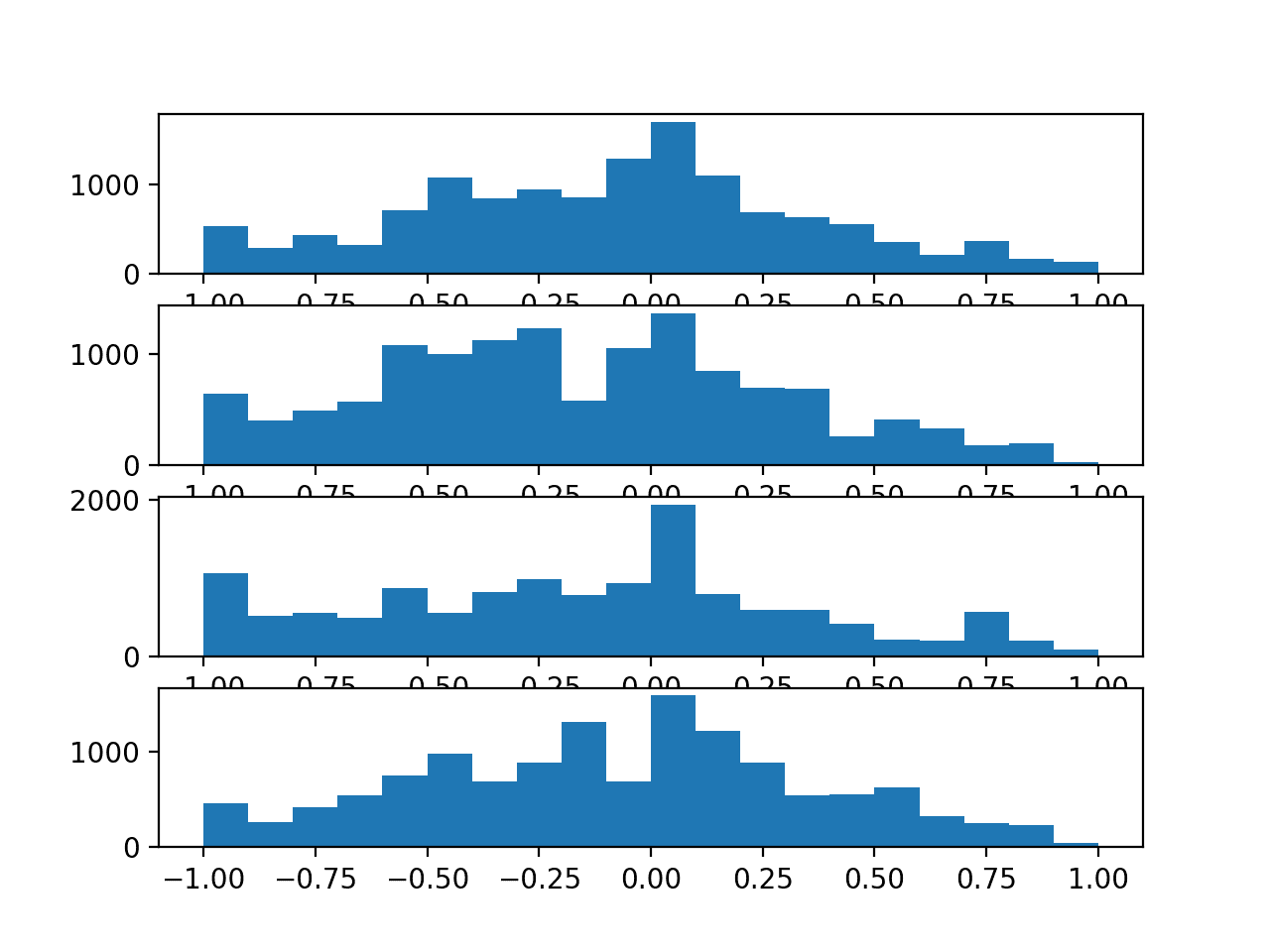
Histograms for the sensor strength values for each anchor point

Finally, a histogram of the sequence lengths is created.

We can see clusters of sequences with lengths around 25, 40, and 60. We can also see that if we wanted to trim long sequences that a maximum length of around 70 time steps might be appropriate. The smallest length appears to be 19.

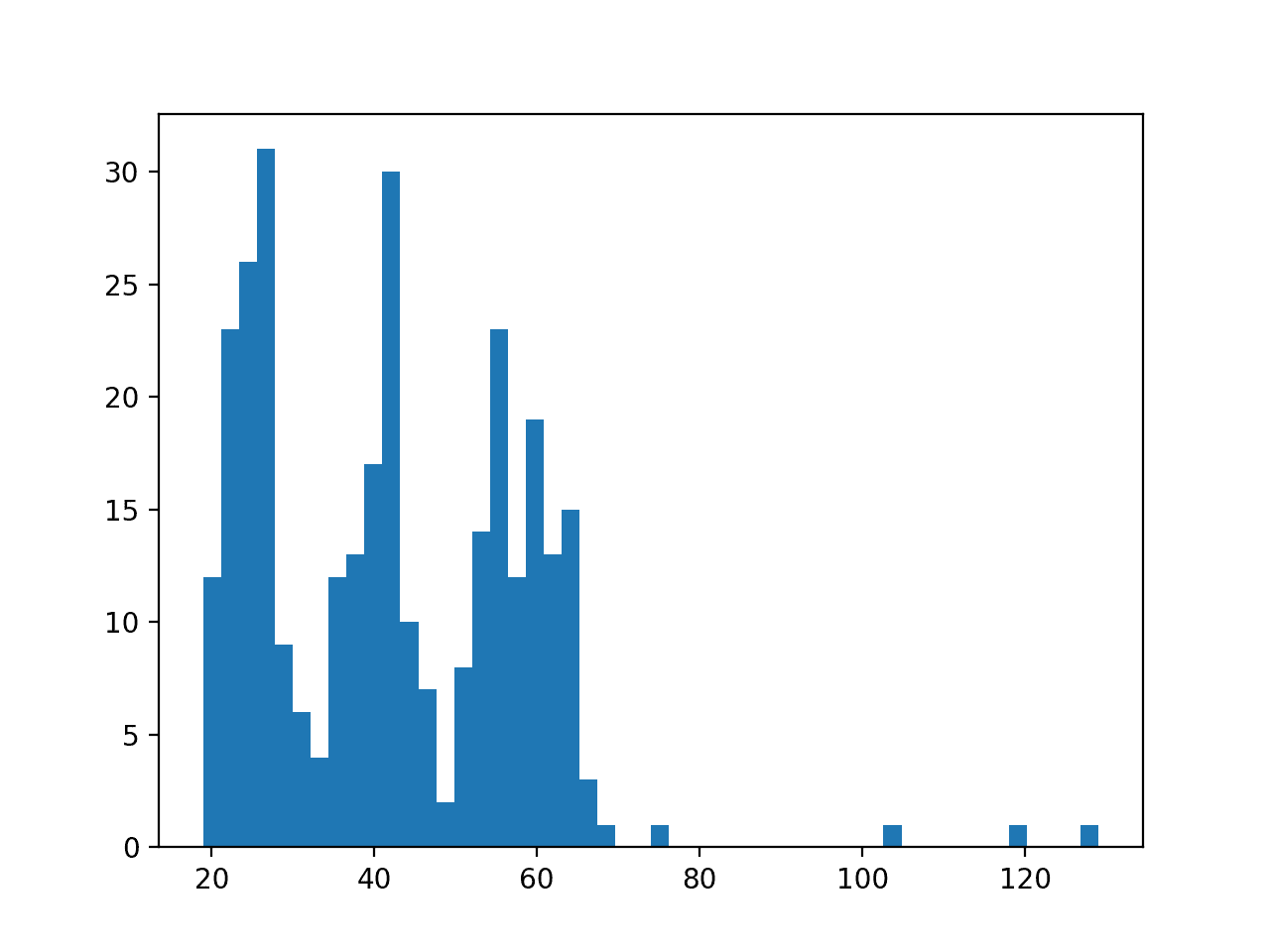
Histogram of sensor strength sequence lengths

Time Series Plots

We are working with time series data, so it is important that we actually review some examples of the sequences.

We can group traces by their path and plot an example of one trace for each path. The expectation is that traces for different paths may look different in some way.

We can also plot each series from one trace along with the trend predicted by a linear regression model. This will make any trends in the series obvious.

We can fit a linear regression for a given series using the lstsq() NumPy Function.

The function regress() below takes a series as a single variable, fits a linear regression model via least squares, and predicts the output for each time step returning a sequence that captures the trend in the data.

We can use the function to plot the trend for the time series for each variable in a single trace.

Tying all of this together, the complete example is listed below.

Running the example creates a plot containing six figures, one for each of the six paths. A given figure shows the line plots of a single trace with the four variables of the trace, one for each anchor point.

Perhaps the chosen traces are representative of each path, perhaps not.

We can see some clear differences with regards to:

• The grouping of variables over time. Pairs of variables may be grouped together or all variables may be grouped together at a given time.
• The trend of variables over time. Variables bunch together towards the middle or spread apart towards the extremes.

Ideally, if these changes in behavior are predictive, a predictive model must extract these features, or be presented with a summary of these features as input.

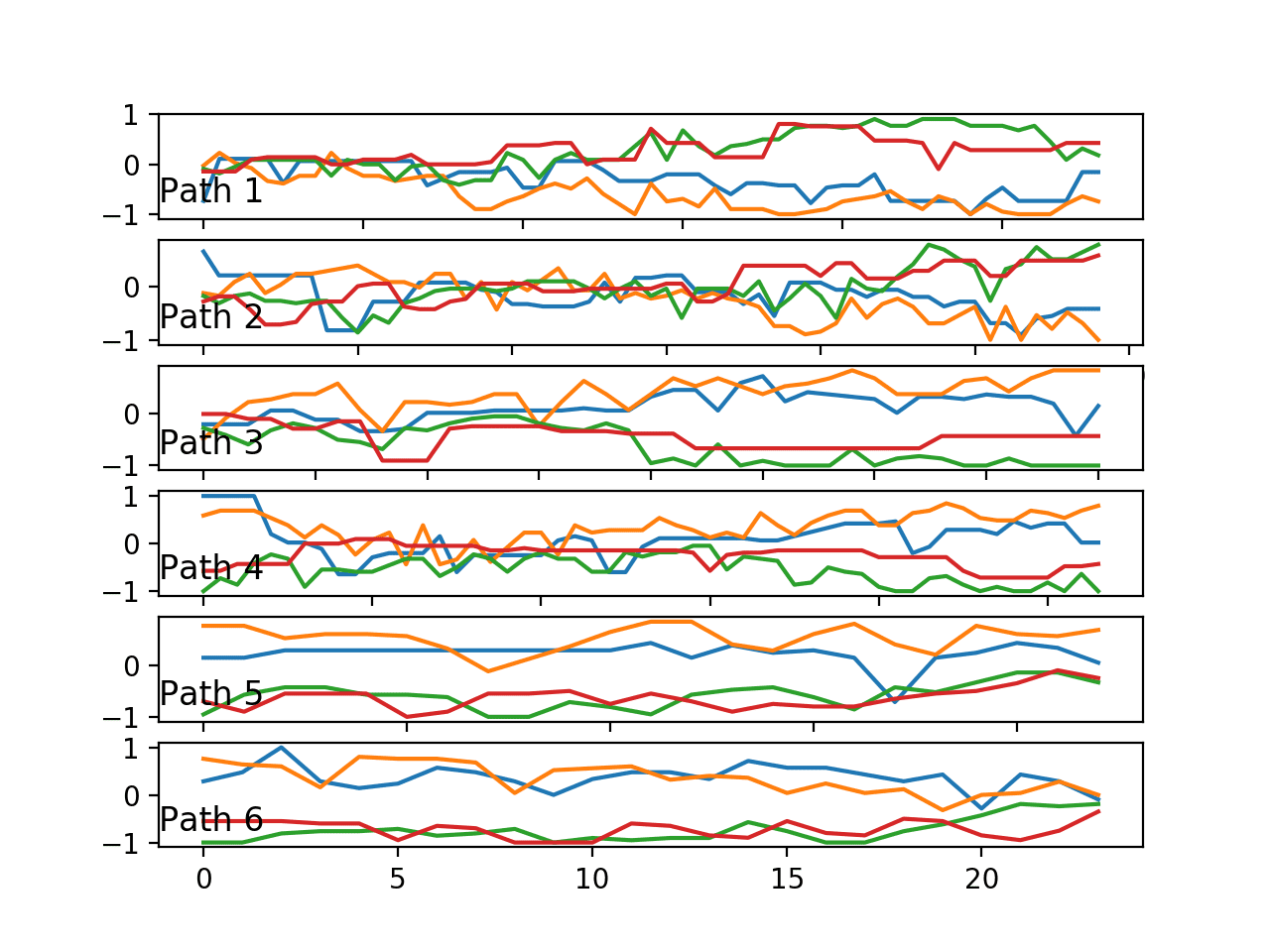
Line plots of one trace (4 variables) for each of the six paths.

A second plot is created showing the line plots for the four series in a single trace along with the trend lines.

We can see that, at least for this trace, there is a clear trend in the sensor strength data as the user moves around the environment. This may suggest the opportunity to make the data stationary prior to modeling or using the trend for each series in a trace (observations or coefficients) as inputs to a predictive model.

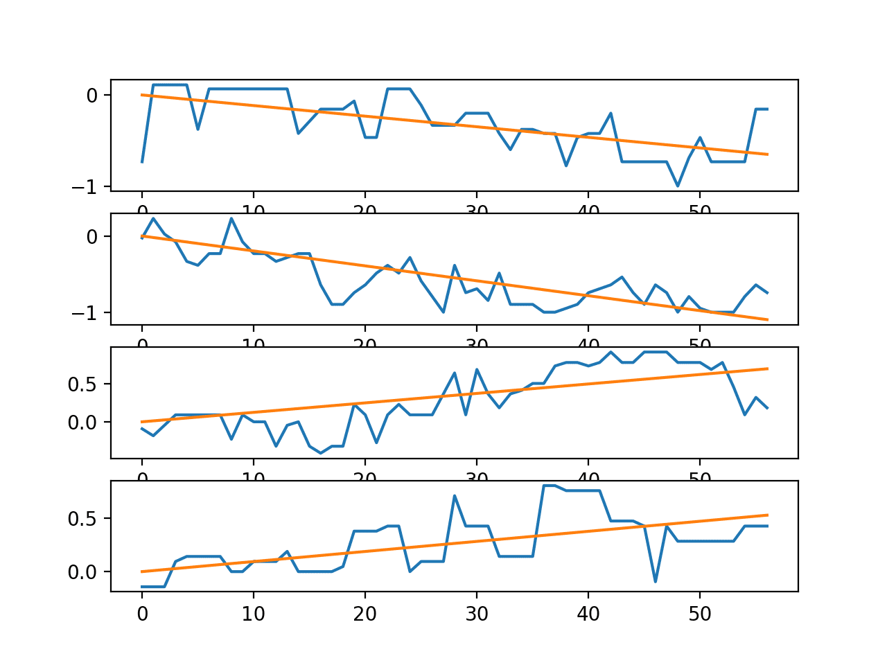
Line plots for the time series in a single trace with trend lines

Model Evaluation

There are many ways to fit and evaluate a model on this data.

Classification accuracy seems like a good first-cut evaluation metric given the balance of the classes. More nuance can be sought in the future by predicting probabilities and exploring thresholds on an ROC curve.

I see two main themes in using this data:

• Same Room: Can a model trained on traces in a room predict the outcome of new traces in that room?
• Different Room: Can a model trained on traces in one or two rooms predict the outcome of new traces in a different room?

The ES1 and ES2 cases described in the paper and summarized above explore these questions and provide a useful starting point.

First, we must partition the loaded traces and targets into the three groups.

In the case of ES1, we can use k-fold cross-validation where k=5 to use the same ratio from the paper and the repeated evaluation provides some robustness to the evaluation.

We can use the cross_val_score() function from scikit-learn to evaluate a model and then calculate the mean and standard deviation of the scores.

In the case of ES2, we can fit the model on datasets 1 and 2 and test model skill on dataset 3 directly.

Data Preparation

There is flexibility in how the input data is framed for the prediction problem.

Two approaches come to mind:

• Automatic Feature Learning. Deep neural networks are capable of automatic feature learning and recurrent neural networks can directly support multivariate multi-step input data. A recurrent neural network could be used, such as an LSTM or 1D CNN. The sequences could be padded to be the same length, such as 70 time steps, and a Masking layer could be used to ignore the padded time steps.
• Feature Engineering. Alternately, the variable length sequences could be summarized as a single fixed length vector and provided to standard machine learning models for prediction. This would require careful feature engineering in order to provide a sufficient description of the trace for the model to learn a mapping to the output class.

Both are interesting approaches.

As a first pass, we will prepare the more traditional fixed-length vector input via manual feature engineering.

Below are some ideas on features that could be included in the vector:

• First, middle, or last n observations for a variable.
• Mean or standard deviation for the first, middle, or last n observations for a variable.
• Difference between the last and first n’th observations
• Differenced first, middle, or last n observations for a variable.
• Linear regression coefficients of all, first, middle, or last n observations for a variable.
• Linear regression predicted trend of first, middle, or last n observations for a variable.

Additionally, data scaling is probably not required of the raw values as the data has already been scaled to the range -1 to 1. Scaling may be required if new features are added with different units.

Some of the variables do show some trend, suggesting that perhaps a differencing of the variables may help in teasing out a signal.

The distribution of each variable is nearly Gaussian, so some algorithms may benefit from standardization, or perhaps even a Box-Cox transform.

Algorithm Spot-Check

In this section, we will spot-check the default configuration for a suite of standard machine learning algorithms with different sets of engineered features.

Spot-checking is a useful technique to flush out quickly whether there is any signal to be learned in the mapping between inputs and outputs with engineered features as most of the tested methods will pick something up. The method can also suggest methods that might be worth further investigating.

A downside is that each method is not given its best chance (configuration) to show what it can do on the problem, meaning any methods that are further investigated will be biased by the first results.

In these tests, we will look at a suite of six different types of algorithms, specifically:

• Logistic Regression.
• k-Nearest Neighbors.
• Decision Tree.
• Support Vector Machine.
• Random Forest.
• Gradient Boosting Machine.

We will test the default configurations of these methods on features that focus on the end of the time series variables as they are likely the most predictive of whether a room transition will occur or not.

Last n Observations

The last n observations are likely to be predictive of whether the movement leads to a transition in rooms.

The smallest number of time steps in the trace data is 19, therefore, we will use n=19 as a starting point.

The function below named create_dataset() will create a fixed-length vector using the last n observations from each trace in a flat one-dimensional vector, then add the target as the last element of the vector.

This flattening of the trace data is required for simple machine learning algorithms.

We can load the dataset as before and sort it into the datasets 1, 2, and 3 as described in the “Model Evaluation” section.

We can then call the create_dataset() function to create the datasets required for the ES1 and ES2 cases, specifically ES1 combines datasets 1 and 2, whereas ES2 uses datasets 1 and 2 as a training set and dataset 3 as a test set.

The complete example is listed below.

Running the example creates three new CSV files, specifically ‘es1.csv‘, ‘es2_train.csv‘, and ‘es2_test.csv‘ for the ES1 and ES2 cases respectively.

The shapes of these datasets are also summarized.

Next, we can evaluate models on the ES1 dataset.

After some testing, it appears that standardizing the dataset results in better model skill for those methods that rely on distance values (KNN and SVM) and generally has no effect on other methods. Therefore a Pipeline is used to evaluate each algorithm that first standardizes the dataset.

The complete example of spot checking algorithms on the new dataset is listed below.

Running the example prints the estimated performance of each algorithm, including the mean and standard deviation over 5-fold cross-validation.

Note: Your results may vary given the stochastic nature of the algorithm or evaluation procedure, or differences in numerical precision. Consider running the example a few times and compare the average outcome.

The results suggest SVM might be worth looking at in more detail at 58% accuracy.

The results are also presented as box-and-whisker plots showing the distribution of scores.

Again, SVM appears to have good average performance and tight variance.

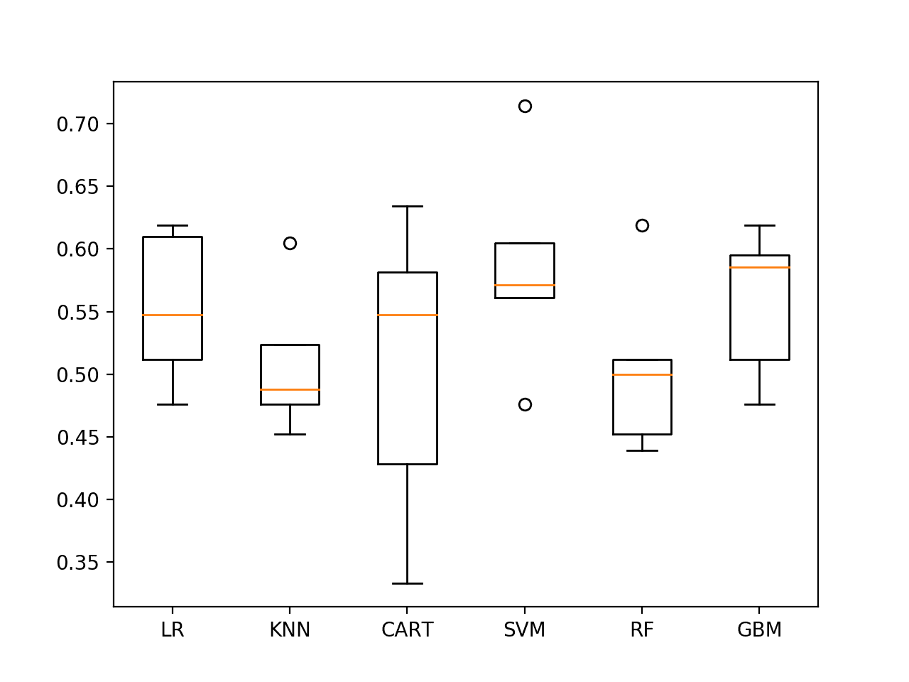
Spot-check Algorithms on ES1 with last 19 observations

Last n Observations With Padding

We can pad each trace to a fixed length.

This will then provide the flexibility to include more of the prior n observations in each sequence. The choice of n must also be balanced with the increase in padded values added to shorter sequences that in turn may negatively impact the performance of the model on those sequences.

We can pad each sequence by adding the 0.0 value to the beginning of each variable sequence until a maximum length, e.g. 200 time steps, is reached. We can do this using the pad() NumPy function.

The updated version of the create_dataset() function with padding support is below.

We will try n=25 to include 25 of the last observations in each sequence in each vector. This value was found with a little trial and error, although you may want to explore whether other configurations result in better skill.

Running the script again with the new function creates updated CSV files.

Note: Your results may vary given the stochastic nature of the algorithm or evaluation procedure, or differences in numerical precision. Consider running the example a few times and compare the average outcome.

Again, re-running the spot-check script on the data results in a small lift in model skill for SVM and also suggests that KNN might be worth investigating further.

The box plots for KNN and SVM show good performance and relatively tight standard deviations.

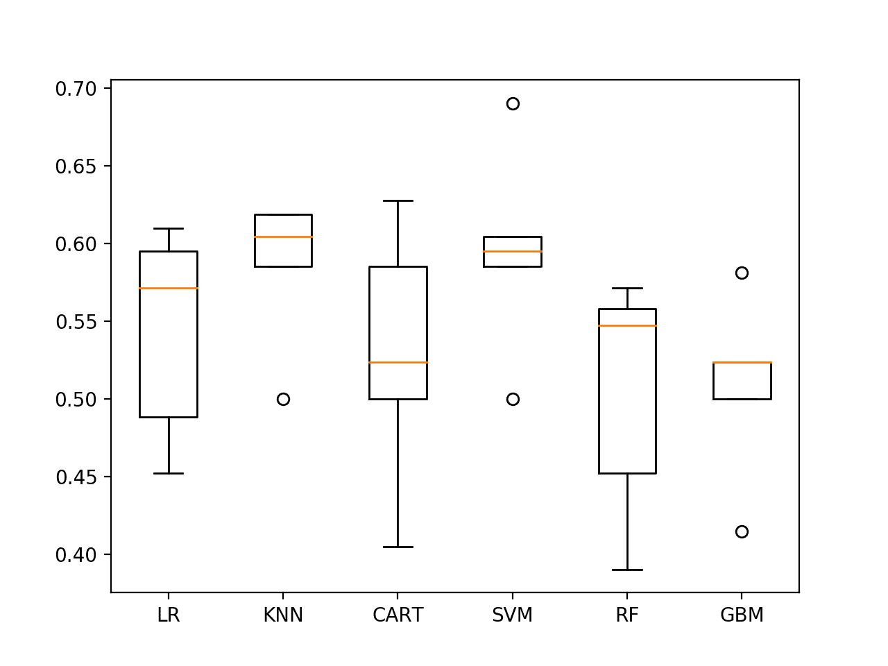
Spot-check Algorithms on ES1 with last 25 observations

We can update the spot-check to grid search a suite of k values for the KNN algorithm to see if the skill of the model can be further improved with a little tuning.

The complete example is listed below.

Running the example prints the mean and standard deviation of the accuracy with k values from 1 to 21.

Note: Your results may vary given the stochastic nature of the algorithm or evaluation procedure, or differences in numerical precision. Consider running the example a few times and compare the average outcome.

We can see that a k=7 results in the best skill of 62.872%.

The box and whisker plots of accuracy scores for k values show that k values around seven, such as five and six, also produce stable and well-performing models on the dataset.

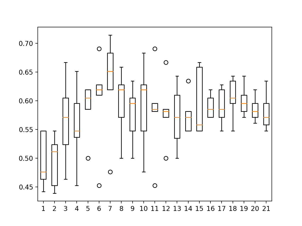
Spot-check KNN neighbors on ES1 with last 25 observations

Evaluate KNN on ES2

Now that we have some idea of a representation (n=25) and a model (KNN, k=7) that have some skill over a random prediction, we can test the approach on the harder ES2 dataset.

Each model is trained on the combination of dataset 1 and 2, then evaluated on dataset 3. The k-fold cross-validation procedure is not used, so we would expect the scores to be noisy.

The complete spot checking of algorithms for ES2 is listed below.

Running the example reports the model accuracy on the ES2 scenario.

Note: Your results may vary given the stochastic nature of the algorithm or evaluation procedure, or differences in numerical precision. Consider running the example a few times and compare the average outcome.

We can see that KNN does well and that the KNN with seven neighbors found to perform well on ES1 also performs well on ES2.

A bar chart of the accuracy scores helps to make the relative difference in performance between the methods clearer.

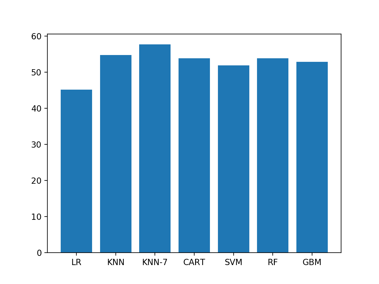
Bar chart of model accuracy on ES2

The chosen representation and model configurations do have skill over a naive prediction with 50% accuracy.

Further tuning may result in models with better skill, and we are a long way from the 95% and 89% accuracy reported in the paper on ES1 and ES2 respectively.

Extensions

This section lists some ideas for extending the tutorial that you may wish to explore.

• Data Preparation. There is a lot of opportunity to explore further data preparation methods such as normalization, differencing, and power transforms.
• Feature Engineering. Further feature engineering may result in better performing models, such as statistics for both the start, middle, and end of each sequence as well as trend information.
• Tuning. Only the KNN algorithm was given the opportunity for tuning; other models such as gradient boosting may benefit from fine tuning of hyperparameters.
• RNNs. This sequence classification task seems well suited to recurrent neural networks such as LSTMs that support variable length multivariate inputs. Some preliminary testing on this dataset (by myself) showed highly unstable results, but more extensive investigation may give better and even superior results.

If you explore any of these extensions, I’d love to know.

Further Reading

This section provides more resources on the topic if you are looking to go deeper.

Papers

• Predicting user movements in heterogeneous indoor environments by reservoir computing, 2011.
• An experimental characterization of reservoir computing in ambient assisted living applications, 2014.

API

• sklearn.model_selection.cross_val_score API
• numpy.linalg.lstsq API
• numpy.pad API

Articles

• Indoor User Movement Prediction from RSS data Data Set, UCI Machine Learning Repository
• Predicting User Movements in Heterogeneous Indoor Environments by Reservoir Computing, Paolo Barsocchi homepage.
• Indoor User Movement Prediction from RSS data Data Set, Laurae [French].

Summary

In this tutorial, you discovered the indoor movement prediction time series classification problem and how to engineer features and evaluate machine learning algorithms for the problem.

Specifically, you learned:

• The time series classification problem of predicting the movement between rooms based on sensor strength.
• How to investigate the data in order to better understand the problem and how to engineer features from the raw data for predictive modeling.
• How to spot check a suite of classification algorithms and tune one algorithm to further lift performance on the problem.

Do you have any questions?
Ask your questions in the comments below and I will do my best to answer.

Develop Deep Learning models for Time Series Today!

Develop Your Own Forecasting models in Minutes

...with just a few lines of python code

Discover how in my new Ebook:
Deep Learning for Time Series Forecasting

It provides self-study tutorials on topics like:
CNNs, LSTMs, Multivariate Forecasting, Multi-Step Forecasting and much more...

Finally Bring Deep Learning to your Time Series Forecasting Projects

Skip the Academics. Just Results.

See What's Inside