A large portion of the field of statistics is concerned with methods that assume a Gaussian distribution: the familiar bell curve.
If your data has a Gaussian distribution, the parametric methods are powerful and well understood. This gives some incentive to use them if possible. Even if your data does not have a Gaussian distribution.
It is possible that your data does not look Gaussian or fails a normality test, but can be transformed to make it fit a Gaussian distribution. This is more likely if you are familiar with the process that generated the observations and you believe it to be a Gaussian process, or the distribution looks almost Gaussian, except for some distortion.
In this tutorial, you will discover the reasons why a Gaussian-like distribution may be distorted and techniques that you can use to make a data sample more normal.
After completing this tutorial, you will know:
How to consider the size of the sample and whether the law of large numbers may help improve the distribution of a sample.
How to identify and remove extreme values and long tails from a distribution.
Power transforms and the Box-Cox transform that can be used to control for quadratic or exponential distributions.
Kick-start your project with my new book Statistics for Machine Learning, including step-by-step tutorials and the Python source code files for all examples.
Let’s get started.
How to Transform Data to Better Fit The Normal Distribution Photo by duncan_idaho_2007, some rights reserved.
Tutorial Overview
This tutorial is divided into 7 parts; they are:
Gaussian and Gaussian-Like
Sample Size
Data Resolution
Extreme Values
Long Tails
Power Transforms
Use Anyway
Need help with Statistics for Machine Learning?
Take my free 7-day email crash course now (with sample code).
Click to sign-up and also get a free PDF Ebook version of the course.
Gaussian and Gaussian-Like
There may be occasions when you are working with a non-Gaussian distribution, but wish to use parametric statistical methods instead of nonparametric methods.
For example, you may have a data sample that has the familiar bell-shape, meaning that it looks Gaussian, but it fails one or more statistical normality tests. This suggests that the data may be Gaussian-like. You would prefer to use parametric statistics in this situation given that better statistical power and because the data is clearly Gaussian, or could be, after the right data transform.
There are many reasons why the dataset may not be technically Gaussian. In this post, we will look at some simple techniques that you may be able to use to transform a data sample with a Gaussian-like distribution into a Gaussian distribution.
There is no silver bullet for this process; some experimentation and judgment may be required.
Sample Size
One common reason that a data sample is non-Gaussian is because the size of the data sample is too small.
Many statistical methods were developed where data was scarce. Hence, the minimum. number of samples for many methods may be as low as 20 or 30 observations.
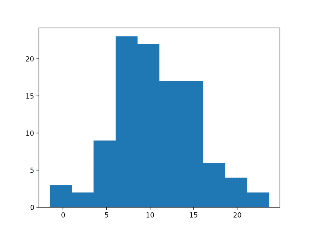
Nevertheless, given the noise in your data, you may not see the familiar bell-shape or fail normality tests with a modest number of samples, such as 50 or 100. If this is the case, perhaps you can collect more data. Thanks to the law of large numbers, the more data that you collect, the more likely your data will be able to used to describe the underlying population distribution.
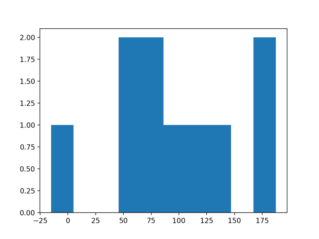
To make this concrete, below is an example of a plot of a small sample of 50 observations drawn from a Gaussian distribution with a mean of 100 and a standard deviation of 50.
1
2
3
4
5
6
7
8
9
10
11
# histogram plot of a small sample
from numpy.random import seed
from numpy.random import randn
from matplotlib import pyplot
# seed the random number generator
seed(1)
# generate a univariate data sample
data=50*randn(50)+100
# histogram
pyplot.hist(data)
pyplot.show()
Running the example creates a histogram plot of the data showing no clear Gaussian distribution, not even Gaussian-like.
Histogram Plot of Very Small Data Sample
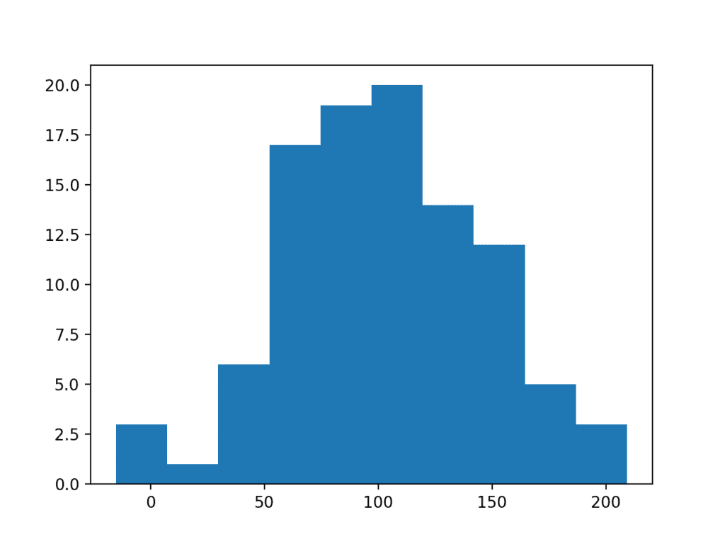
Increasing the size of the sample from 50 to 100 can help to better expose the Gaussian shape of the data distribution.
1
2
3
4
5
6
7
8
9
10
11
# histogram plot of a small sample
from numpy.random import seed
from numpy.random import randn
from matplotlib import pyplot
# seed the random number generator
seed(1)
# generate a univariate data sample
data=50*randn(100)+100
# histogram
pyplot.hist(data)
pyplot.show()
Running the example, we can better see the Gaussian distribution of the data that would pass both statistical tests and eye-ball checks.
Histogram Plot of Larger Data Sample
Data Resolution
Perhaps you expect a Gaussian distribution from the data, but no matter the size of the sample that you collect, it does not materialize.
A common reason for this is the resolution that you are using to collect the observations. The distribution of the data may be obscured by the chosen resolution of the data or the fidelity of the observations. There may be many reasons why the resolution of the data is being modified prior to modeling, such as:
The configuration of the mechanism making the observation.
The data is passing through a quality-control process.
The resolution of the database used to store the data.
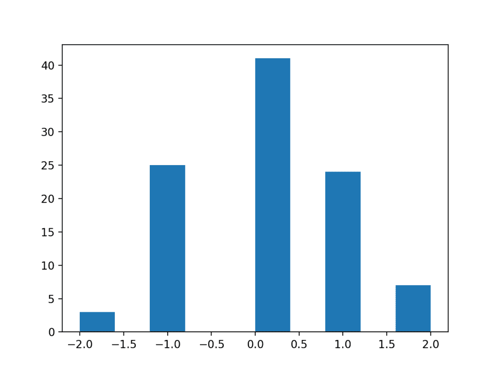
To make this concrete, we can make a sample of 100 random Gaussian numbers with a mean of 0 and a standard deviation of 1 and remove all of the decimal places.
1
2
3
4
5
6
7
8
9
10
11
12
13
# histogram plot of a low res sample
from numpy.random import seed
from numpy.random import randn
from matplotlib import pyplot
# seed the random number generator
seed(1)
# generate a univariate data sample
data=randn(100)
# remove decimal component
data=data.round(0)
# histogram
pyplot.hist(data)
pyplot.show()
Running the example results in a distribution that appears discrete although Gaussian-like. Adding the resolution back to the observations would result in a fuller distribution of the data.
Histogram Plot of a Low Resolution Data Sample
Extreme Values
A data sample may have a Gaussian distribution, but may be distorted for a number of reasons.
A common reason is the presence of extreme values at the edge of the distribution. Extreme values could be present for a number of reasons, such as:
Measurement error.
Missing data.
Data corruption.
Rare events.
In such cases, the extreme values could be identified and removed in order to make the distribution more Gaussian. These extreme values are often called outliers.
This may require domain expertise or consultation with a domain expert in order to both design the criteria for identifying outliers and then removing them from the data sample and all data samples that you or your model expect to work with in the future.
We can demonstrate how easy it is to have extreme values disrupt the distribution of data.
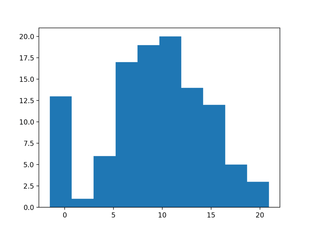
The example below creates a data sample with 100 random Gaussian numbers scaled to have a mean of 10 and a standard deviation of 5. An additional 10 zero-valued observations are then added to the distribution. This can happen if missing or corrupt values are assigned the value of zero. This is a common behavior in publicly available machine learning datasets; for example.
1
2
3
4
5
6
7
8
9
10
11
12
13
14
15
# histogram plot of data with outliers
from numpy.random import seed
from numpy.random import randn
from numpy import zeros
from numpy import append
from matplotlib import pyplot
# seed the random number generator
seed(1)
# generate a univariate data sample
data=5*randn(100)+10
# add extreme values
data=append(data,zeros(10))
# histogram
pyplot.hist(data)
pyplot.show()
Running the example creates and plots the data sample. You can clearly see how the unexpected high frequency of zero-valued observations disrupts the distribution.
Histogram Plot of Data Sample With Extreme Values
Long Tails
Extreme values can manifest in many ways. In addition to an abundance of rare events at the edge of the distribution, you may see a long tail on the distribution in one or both directions.
In plots, this can make the distribution look like it is exponential, when in fact it might be Gaussian with an abundance of rare events in one direction.
You could use simple threshold values, perhaps based on the number of standard deviations from the mean, to identify and remove long tail values.
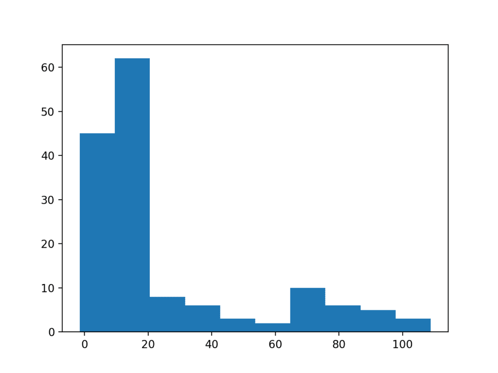
We can demonstrate this with a contrived example. The data sample contains 100 Gaussian random numbers with a mean of 10 and a standard deviation of 5. An additional 50 uniformly random values in the range 10-to-110 are added. This creates a long tail on the distribution.
1
2
3
4
5
6
7
8
9
10
11
12
13
14
15
16
# histogram plot of data with a long tail
from numpy.random import seed
from numpy.random import randn
from numpy.random import rand
from numpy import append
from matplotlib import pyplot
# seed the random number generator
seed(1)
# generate a univariate data sample
data=5*randn(100)+10
tail=10+(rand(50)*100)
# add long tail
data=append(data,tail)
# histogram
pyplot.hist(data)
pyplot.show()
Running the example you can see how the long tail distorts the Gaussian distribution and makes it look almost exponential or perhaps even bimodal (two bumps).
Histogram Plot of Data Sample With Long Tail
We can use a simple threshold, such as a value of 25, on this dataset as a cutoff and remove all observations higher than this threshold. We did choose this threshold with prior knowledge of how the data sample was contrived, but you can imagine testing different thresholds on your own dataset and evaluating their effect.
1
2
3
4
5
6
7
8
9
10
11
12
13
14
15
16
17
18
# histogram plot of data with a long tail
from numpy.random import seed
from numpy.random import randn
from numpy.random import rand
from numpy import append
from matplotlib import pyplot
# seed the random number generator
seed(1)
# generate a univariate data sample
data=5*randn(100)+10
tail=10+(rand(10)*100)
# add long tail
data=append(data,tail)
# trim values
data=[xforxindata ifx<25]
# histogram
pyplot.hist(data)
pyplot.show()
Running the code shows how this simple trimming of the long tail returns the data to a Gaussian distribution.
Histogram Plot of Data Sample With a Truncated Long Tail
Power Transforms
The distribution of the data may be normal, but the data may require a transform in order to help expose it.
For example, the data may have a skew, meaning that the bell in the bell shape may be pushed one way or another. In some cases, this can be corrected by transforming the data via calculating the square root of the observations.
Alternately, the distribution may be exponential, but may look normal if the observations are transformed by taking the natural logarithm of the values. Data with this distribution is called log-normal.
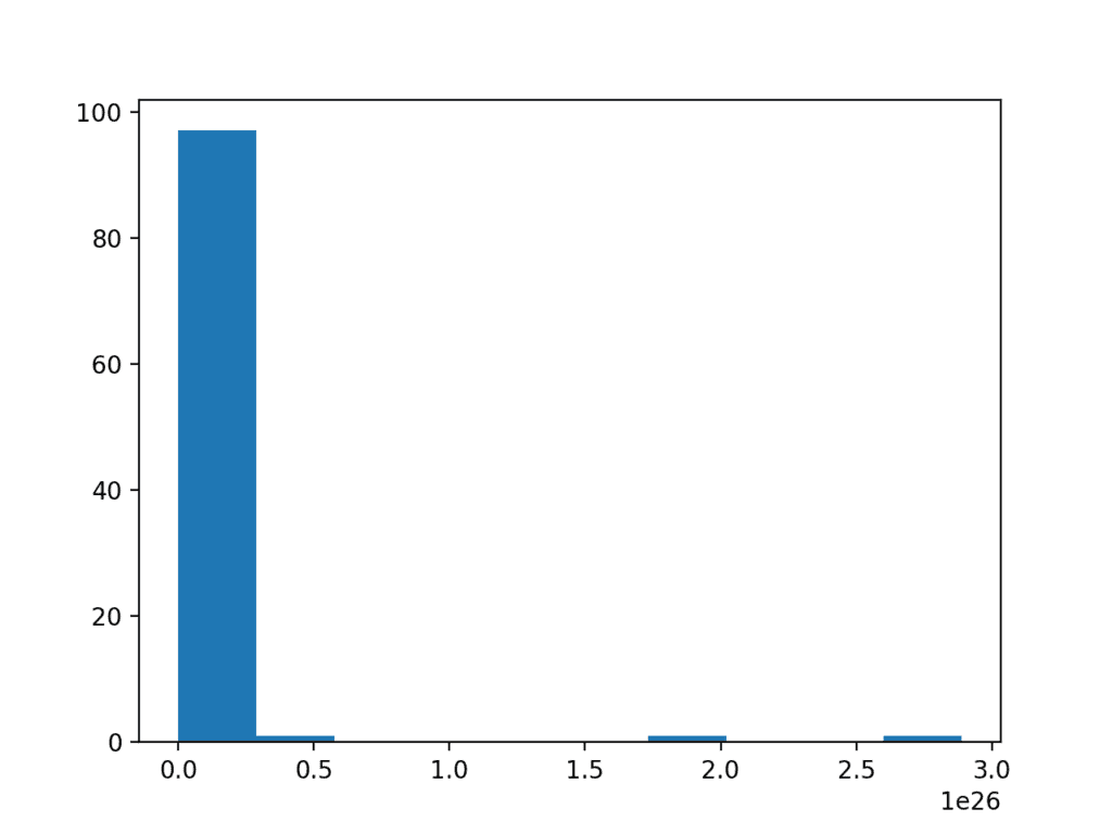
To make this concrete, below is an example of a sample of Gaussian numbers transformed to have an exponential distribution.
1
2
3
4
5
6
7
8
9
10
11
12
13
14
# log-normal distribution
from numpy.random import seed
from numpy.random import randn
from numpy import exp
from matplotlib import pyplot
# seed the random number generator
seed(1)
# generate two sets of univariate observations
data=5*randn(100)+50
# transform to be exponential
data=exp(data)
# histogram
pyplot.hist(data)
pyplot.show()
Running the example creates a histogram showing the exponential distribution. It is not obvious that the data is in fact log-normal.
Histogram of a Log Normal Distribution
Taking the square root and the logarithm of the observation in order to make the distribution normal belongs to a class of transforms called power transforms. The Box-Cox method is a data transform method that is able to perform a range of power transforms, including the log and the square root. The method is named for George Box and David Cox.
More than that, it can be configured to evaluate a suite of transforms automatically and select a best fit. It can be thought of as a power tool to iron out power-based change in your data sample. The resulting data sample may be more linear and will better represent the underlying non-power distribution, including Gaussian.
The boxcox() SciPy function implements the Box-Cox method. It takes an argument, called lambda, that controls the type of transform to perform.
Below are some common values for lambda:
lambda = -1. is a reciprocal transform.
lambda = -0.5 is a reciprocal square root transform.
lambda = 0.0 is a log transform.
lambda = 0.5 is a square root transform.
lambda = 1.0 is no transform.
For example, because we know that the data is lognormal, we can use the Box-Cox to perform the log transform by setting lambda explicitly to 0.
1
2
# power transform
data=boxcox(data,0)
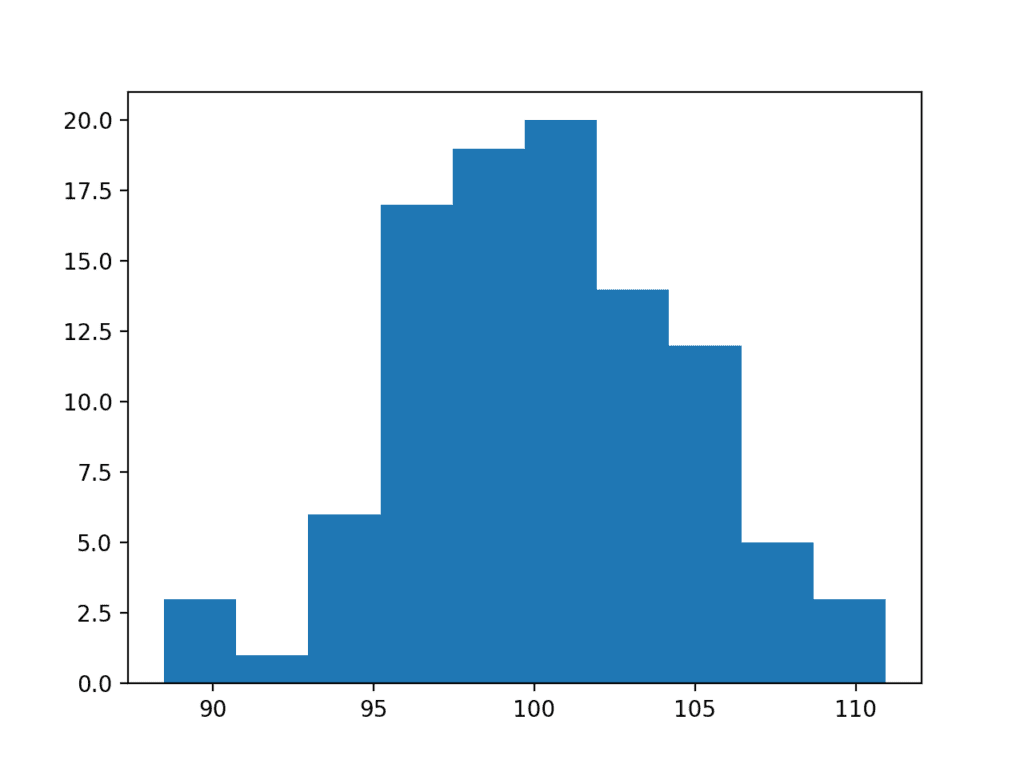
The complete example of applying the Box-Cox transform on the exponential data sample is listed below.
1
2
3
4
5
6
7
8
9
10
11
12
13
14
15
16
17
# box-cox transform
from numpy.random import seed
from numpy.random import randn
from numpy import exp
from scipy.stats import boxcox
from matplotlib import pyplot
# seed the random number generator
seed(1)
# generate two sets of univariate observations
data=5*randn(100)+100
# transform to be exponential
data=exp(data)
# power transform
data=boxcox(data,0)
# histogram
pyplot.hist(data)
pyplot.show()
Running the example performs the Box-Cox transform on the data sample and plots the result, clearly showing the Gaussian distribution.
Histogram Plot of Box Cox Transformed Exponential Data Sample
A limitation of the Box-Cox transform is that it assumes that all values in the data sample are positive.
An alternative method that does not make this assumption is the Yeo-Johnson transformation.
Use Anyway
Finally, you may wish to treat the data as Gaussian anyway, especially if the data is already Gaussian-like.
In some cases, such as the use of parametric statistical methods, this may lead to optimistic findings.
In other cases, such as machine learning methods that make Gaussian expectations on input data, you may still see good results.
This is a choice you can make, as long as you are aware of the possible downsides.
Extensions
This section lists some ideas for extending the tutorial that you may wish to explore.
List 3 possible additional ways that a Gaussian distribution may have been distorted
Develop a data sample and experiment with the 5 common values for lambda in the Box-Cox transform.
Load a machine learning dataset where at least one variable has a Gaussian-like distribution and experiment.
If you explore any of these extensions, I’d love to know.
Further Reading
This section provides more resources on the topic if you are looking to go deeper.
In this tutorial, you discovered the reasons why a Gaussian-like distribution may be distorted and techniques that you can use to make a data sample more normal.
Specifically, you learned:
How to consider the size of the sample and whether the law of large numbers may help improve the distribution of a sample.
How to identify and remove extreme values and long tails from a distribution.
Power transforms and the Box-Cox transform that can be used to control for quadratic or exponential distributions.
Do you have any questions?
Ask your questions in the comments below and I will do my best to answer.
Dear Dr Jason,
Do you have to do any further testing after the data has been transformed?
That is suppose a Box-Cox transformation is performed on the data to have a symmetrical Gaussian appearance. What are the further tests to ensure that the transformed data is Gaussian.
Another question is that the Poisson distribution is a distribution of discrete values rather than continuous values. A Poisson distribution can have a symmetrical histogram. Could machine learning techniques relying on the assumption that the data is guassian apply to Poisson distribution?
Poisson is not always symmetric. In the case that it is, many algorithms that assume gaussian are robust enough to work with other symmetric distributions without failing badly.
As Ravi said, vert well explained!
Now, if I want to use this method on real world data, do I need to look at every feature distribution and try to transform it into Gaussian using these methods?
Mr. Brownlee hello.
I am trying to make an algorithm in Python taking data from a fits file named “NGC5055_HI_lab.fits
and making them another fits file f.e “test.fits”.
So far i can’t do something.
My algorithm so far is the following…
from matplotlib import pyplot as mp
import numpy as np
import astropy.io.fits as af
cube=af.open (‘NGC5055_HI_lab.fits’)[0]
mo=np.mean(cube.data)
s=np.var(cube.data)
σ=np.std(cube.data)
amp=1/(σ*np.sqrt(2*3.14))
cube.data=amp*np.exp(-np.power(cube.data-mo,2.)/(2*np.power(s,2.)))
cube.writeto(‘test.fits, overwrite=True)
First of all, thank you very much for your helpful blog posts.
I just have a specific question for my feature variables, and I hope you can help me. I have multiple features as input for machine learning. However, my features have very different distributions. Some of them are normally distributed but some are highly skewed. Is it valid to make different types of transformations for different features? For example, some features will be log transformed, but some i can retain the original?
Hi, everything is so helpful, thank you very much. I have a doubt related to this subject. what should we do ıf the variable not have normal distribution across all groups? For example for the man is already normal when the woman is not. But after transformation, it is vise-versa so can I transform the variables separately according to groups.
I hope I could explain what is my problem.
i have a non-normally distributed data. if i run Pandas Spearman correlation, would it automatically transform data to ordinal or do I need to transform the data to ordinal first?
I landed at this page post reading your book on Python Mastery and I must say the book was awesome. Thanks for coming with such lucid ebooks.
I am a begineer in data science and have a basic question. If we want to build multiple models so to chose the best one depending on accuracy, do we need to tranform all input variables into normal distribution. I intend to use regression various linera and non linear alg such as Log reg, SVM, NN, DT, etc. on the data. If yes, which alg i particular shd we gor for normally distributed variables?
Hi Jason,
Learnt one or two things in this post.
What’s the best way to transform features that have negative and positive values? Tried to use boxcox function but it doesn’t support negative values.
Thanks
It is a very good explanation thanks for taking the time detail it out.I had one ? how do you know that the data is log normal(near the histogram image of log normal distribution).please elobarate.
Thanks for the detailed explanation. I found this article to be really concise as to what transformation to choose for your situation/ level of skew: https://www.anatomisebiostats.com/biostatistics-blog/transforming-skewed-data
It gets to the point clearly. I find the topic can get a bit murky when you have to make a best choice for your particular data.
Please, if I transform some of the input variables (X) using log for example AND/OR the target variable (Y) using log as well, or even another function, after train the model with fit and do the predictions with predict etc., should I have to invert the results of predictions using the inverse function (log/exp) ?
Could you Sir please just check if the ORDER of my “pipeline” below is correct or not? I mean, to calculate the corrects/real RMSEs at the end of the process.
1. DATASET: X, y
2. SPLIT: X_train, X_test, y_train, y_test
3. Power Transform Y BOXCOX: y_train_BC, y_test_BC
4. Normalization Y MINMAXSCALER: y_train_BC_MMS, y_test_BC_MMS
5. Normalization X MINMAXSCALER: X_train_MMS, X_test_MMS
Ok. Done. But it didn’t improve the RMSEs I got before in the previous step when I power transformed only the output variable (y) and scale transformed both X and y.
I have a set of sensor values [x y]= [467021 478610], [464025 479352], [465688 478515], [464025 478610] etc..around a ground ground truth [x y]= [466111 478611]. I have to find ‘how is the distribution of points by the sensor’ around the ground truth. Which distribution is helpful?
I have plans to work on Expectation Maximization [EM] and clustering using Gaussian mixture model (GMM) Algorithms.
Do i need to transform my input sensor values into Gaussian by applying normalization or any power transform techniques, before applying EM/ GMM algorithm.
OR
Can i use the same [x y] values directly to EM/GMM algorithm without normalization/ standardization techniques as both the values are almost on the scale.
Actually i want to identify the ‘distribution of points’ from the sensor (regarding which distribution the sensor output follows). Also i have the ground truth. The values from sensor are scattered around the ground truth. I need to identify which distribution output of the sensor follows. With this information i have to create a ML model out of that to predict the sensor values as close to the ground truth.
Thats a great post. Loved it!
I have a question regarding dealing with non-gaussian distributed variables/features when it comes to building a ML model.
Suppose i have some features that are not normally distributed, why would that be a problem? (E.g. will it cause non-normally distributed residuals?)
Should we prefer transforming that variables to be normally distributed?
Example:
Its a good/famous practice to use log-scaling for skewed variables, and i know indeed it makes these variables normally distributed, but why is it better for a specific ML algorithm e.g. RandomForest?
I think I’m missing the intuition behind doing this.. would be happy if you can help with this!
It depends on the model. If you use a model that assumes a gaussian distribution, you may get poor or worse results – and it will be a graceful falloff.
Otherwise, perhaps little or no effect. RF will not care.
Thanks this is lovely. I note that scp.boxcox() will select the maximum likelihood estimated value for lambda if you leave the variable blank. Although this did produce a rather strange histogram for data originally drawn from an exponential() distribution.
Could you give me some examples of models that assume a normal distribution of either the response or the predictor variables?
Linear regression assumes only the normality of residuals, not the underlying data. Logistic regression makes no assumptions on the distribution of the independent variables. Neither do tree-based regression methods. Even statistical tests such as t-tests do not assume a normal sample distribution (only a normal population distribution if n is low, but otherwise no distribution is really necessary due to the CLT).
(Would appreciate some additional material that you could link me to for further reading)
Hi! Thanks for an awesome tutorial and your amazing books.
I have a question regarding this specific tutorial about making data more normal.
You’ve touched on the topic of zero-inflated data and emphasized that this often occurs in publicly available datasets. Yet, I haven’t grasped from the tutorial how to make such data fit the normal distribution in an optimal way.
Hi Pavlo…Thank you for your feedback! Please clarify what may be lacking from the procedure presented in the tutorial that is not meeting your needs so that we may better assist you.


Dear Dr Jason,
Do you have to do any further testing after the data has been transformed?
That is suppose a Box-Cox transformation is performed on the data to have a symmetrical Gaussian appearance. What are the further tests to ensure that the transformed data is Gaussian.
Another question is that the Poisson distribution is a distribution of discrete values rather than continuous values. A Poisson distribution can have a symmetrical histogram. Could machine learning techniques relying on the assumption that the data is guassian apply to Poisson distribution?
Thank you,
Anthony of exciting Belfield
You could use these tests:
https://machinelearningmastery.com/a-gentle-introduction-to-normality-tests-in-python/
Poisson is not always symmetric. In the case that it is, many algorithms that assume gaussian are robust enough to work with other symmetric distributions without failing badly.
Well explained.
Thanks a lot Mr. Jason.
Thanks.
As Ravi said, vert well explained!
Now, if I want to use this method on real world data, do I need to look at every feature distribution and try to transform it into Gaussian using these methods?
Thanks!
Depending on the modeling method, yes.
Since Naive bayes assumes distribution to be gaussian, so is it must to transform to gaussian in this case?
Gaussian naive bayes assumes a gaussian distribution, in which case it is a good idea to ensure your data is Gaussian.
Otherwise you can use any distribution like, including the empirical distribution.
Mr. Brownlee hello.
I am trying to make an algorithm in Python taking data from a fits file named “NGC5055_HI_lab.fits
and making them another fits file f.e “test.fits”.
So far i can’t do something.
My algorithm so far is the following…
from matplotlib import pyplot as mp
import numpy as np
import astropy.io.fits as af
cube=af.open (‘NGC5055_HI_lab.fits’)[0]
mo=np.mean(cube.data)
s=np.var(cube.data)
σ=np.std(cube.data)
amp=1/(σ*np.sqrt(2*3.14))
cube.data=amp*np.exp(-np.power(cube.data-mo,2.)/(2*np.power(s,2.)))
cube.writeto(‘test.fits, overwrite=True)
Can you help?
Sounds like a programming problem, not a machine learning question. I recommend posting on stackoverflow.
can i covert all feature to gaussian distribution for linear Distribution
Sorry its linear Reg.
Probably, using something like a quantile transform. But why?
Hi Mr. Brownlee,
First of all, thank you very much for your helpful blog posts.
I just have a specific question for my feature variables, and I hope you can help me. I have multiple features as input for machine learning. However, my features have very different distributions. Some of them are normally distributed but some are highly skewed. Is it valid to make different types of transformations for different features? For example, some features will be log transformed, but some i can retain the original?
Thank you very much.
Yes, prepare each feature separately if required.
Hi, everything is so helpful, thank you very much. I have a doubt related to this subject. what should we do ıf the variable not have normal distribution across all groups? For example for the man is already normal when the woman is not. But after transformation, it is vise-versa so can I transform the variables separately according to groups.
I hope I could explain what is my problem.
Thank you
Perhaps explore if different transforms applied to the data as a whole vs groups vs raw data has an effect on model skill.
Hope you are doing very well.
I am trying to apply a statistical normalization which requires the values to be normally distributed.
I have prepared a short notebook with all the details.
https://nbviewer.jupyter.org/github/diallobakary4/bioinformatics/blob/master/Normatily_test.ipynb
It will be great if someone can help me out.
Thanks
Sorry, I don’t have the capacity to review code, perhaps you can summarize the issue on a sentence or two?
i have a non-normally distributed data. if i run Pandas Spearman correlation, would it automatically transform data to ordinal or do I need to transform the data to ordinal first?
No, you can apply the Spearman correlation directly to the real values.
I want to thank you not only for this tutorial but for the many others that you have published and that I have gained from.
I certainly plan to buy one of your books soon.
Thanks, I really appreciate your support!
Dear Mr. Jason,
Is there any function in python to convert data to lognorm and inverse it back?
Natural log and exp are the inverse functions of each other.
More here:
https://en.wikipedia.org/wiki/Log-normal_distribution
Hi Jason,
I landed at this page post reading your book on Python Mastery and I must say the book was awesome. Thanks for coming with such lucid ebooks.
I am a begineer in data science and have a basic question. If we want to build multiple models so to chose the best one depending on accuracy, do we need to tranform all input variables into normal distribution. I intend to use regression various linera and non linear alg such as Log reg, SVM, NN, DT, etc. on the data. If yes, which alg i particular shd we gor for normally distributed variables?
Thanks and regards,
Heramb
Thanks!
It really depends on the model you’re using. Perhaps try fitting with and without the transform and compare the performance of the model?
Hi Jason,
Learnt one or two things in this post.
What’s the best way to transform features that have negative and positive values? Tried to use boxcox function but it doesn’t support negative values.
Thanks
You can scale the data to be positive, or you can use the Yeo-Johnson transform instead.
Hi Jason,
It is a very good explanation thanks for taking the time detail it out.I had one ? how do you know that the data is log normal(near the histogram image of log normal distribution).please elobarate.
Good question, one way would be to take the log of the data and then review the Q-Q plot or even just a histogram of the data.
Thanks for the detailed explanation. I found this article to be really concise as to what transformation to choose for your situation/ level of skew: https://www.anatomisebiostats.com/biostatistics-blog/transforming-skewed-data
It gets to the point clearly. I find the topic can get a bit murky when you have to make a best choice for your particular data.
Thanks for sharing.
Hi Sir.
Please, if I transform some of the input variables (X) using log for example AND/OR the target variable (Y) using log as well, or even another function, after train the model with fit and do the predictions with predict etc., should I have to invert the results of predictions using the inverse function (log/exp) ?
Thanks much in advance.
Yes, it is a good idea to invert transforms to the predictions before calculating error or using them – to return them to the original units.
Ok. Thanks. One more question please.
Can I use the power transforms (log/exp/etc) in conjunction/together with the scaling transforms (normalization/standardization)?
If so, then should I use the two/both inverse transforms after prediction to get the “real” erros etc?
Thanks much in advance.
Yes, the order of transforms and their reverse is here:
https://machinelearningmastery.com/machine-learning-data-transforms-for-time-series-forecasting/
Ok. Right. I did it. Thanks!
Could you Sir please just check if the ORDER of my “pipeline” below is correct or not? I mean, to calculate the corrects/real RMSEs at the end of the process.
1. DATASET: X, y
2. SPLIT: X_train, X_test, y_train, y_test
3. Power Transform Y BOXCOX: y_train_BC, y_test_BC
4. Normalization Y MINMAXSCALER: y_train_BC_MMS, y_test_BC_MMS
5. Normalization X MINMAXSCALER: X_train_MMS, X_test_MMS
6. Define/compile/FIT/eval Model: X_train_MMS, y_train_BC_MMS
7. PREDICT X_test_MMS: preds_test
8. INVERT Normalization Y preds_test: preds_inverse_MMS
9. INVERT Normalization X: X_test_inverse_MMS
10. INVERT Normalization Y: Y_test_inverse_MMS
11. INVERT Y BoxCox preds_inverse_MMS: preds_inverse_BC
12. INVERT Y BoxCox Y_test_inverse_MMS: Y_test_inverse_BC
13. CALCULATE REAL RMSEs: Y_test_inverse_BC, preds_inverse_BC
Thanks much in advance!
Sorry, I don’t have the capacity to review and debug your work.
Perhaps test it and see?
Ok. I tested it and it seems it’s Ok. I got some RMSEs MUCH better than I was getting before.
I’d like only just make sure the ORDER of my transforms and inverted transforms are correct.
I’ve followed your link below, so I think they are correct…
https://machinelearningmastery.com/machine-learning-data-transforms-for-time-series-forecasting/
Thanks much and best regards!
Well done, that is great to hear!
BTW/In time,
Should/can I use different power transforms and/or different scaling transforms for each input variable (X) ?
Or I must use the same power transforms and/or the same scaling transforms for all the input variables (X) ?
Thanks much in advance.
Great question!
Yes, treat each variable separately.
Ok. Done. But it didn’t improve the RMSEs I got before in the previous step when I power transformed only the output variable (y) and scale transformed both X and y.
Good finding.
Hi All,
I have a set of sensor values [x y]= [467021 478610], [464025 479352], [465688 478515], [464025 478610] etc..around a ground ground truth [x y]= [466111 478611]. I have to find ‘how is the distribution of points by the sensor’ around the ground truth. Which distribution is helpful?
I have plans to work on Expectation Maximization [EM] and clustering using Gaussian mixture model (GMM) Algorithms.
Do i need to transform my input sensor values into Gaussian by applying normalization or any power transform techniques, before applying EM/ GMM algorithm.
OR
Can i use the same [x y] values directly to EM/GMM algorithm without normalization/ standardization techniques as both the values are almost on the scale.
I am beginner in this field. Help me please…..
You could assume the target is the mean of a gaussian and points are some number of stdev from the gaussain, as a modeling exercise.
But what are you trying to achieve exactly? What are you predicting?
Thanks a lot for your response!
Actually i want to identify the ‘distribution of points’ from the sensor (regarding which distribution the sensor output follows). Also i have the ground truth. The values from sensor are scattered around the ground truth. I need to identify which distribution output of the sensor follows. With this information i have to create a ML model out of that to predict the sensor values as close to the ground truth.
I hope you can help me out.
Perhaps you can use a gausaian process to model the density of observed points?
This might give you ideas:
https://machinelearningmastery.com/probability-density-estimation/
Hi Jason,
Thats a great post. Loved it!
I have a question regarding dealing with non-gaussian distributed variables/features when it comes to building a ML model.
Suppose i have some features that are not normally distributed, why would that be a problem? (E.g. will it cause non-normally distributed residuals?)
Should we prefer transforming that variables to be normally distributed?
Example:
Its a good/famous practice to use log-scaling for skewed variables, and i know indeed it makes these variables normally distributed, but why is it better for a specific ML algorithm e.g. RandomForest?
I think I’m missing the intuition behind doing this.. would be happy if you can help with this!
Thanks!
It depends on the model. If you use a model that assumes a gaussian distribution, you may get poor or worse results – and it will be a graceful falloff.
Otherwise, perhaps little or no effect. RF will not care.
Thanks for the quick reply!
So your saying not transforming these variables wont have any effect on the residuals?
I’m saying scaling won’t lift skill on some algorithms, that algorithms like RF are invariant to linear scaling of inputs.
Thanks this is lovely. I note that scp.boxcox() will select the maximum likelihood estimated value for lambda if you leave the variable blank. Although this did produce a rather strange histogram for data originally drawn from an exponential() distribution.
Thanks!
Yes. Intersting.
Hi, Jason!
Could you give me some examples of models that assume a normal distribution of either the response or the predictor variables?
Linear regression assumes only the normality of residuals, not the underlying data. Logistic regression makes no assumptions on the distribution of the independent variables. Neither do tree-based regression methods. Even statistical tests such as t-tests do not assume a normal sample distribution (only a normal population distribution if n is low, but otherwise no distribution is really necessary due to the CLT).
(Would appreciate some additional material that you could link me to for further reading)
how about uniform distribution to normal? i m reading about the box miller transform but its somehow not working on my data..
Hi Vanetoj…Please describe in detail what is “not working” so that we may better assist you.
Hi the 1st and 2nd pictures are no showing currently. Can you fix it?
Hi Hue…We do not see any issues on our side. Perhaps you could try another browser.
Hi! Thanks for an awesome tutorial and your amazing books.
I have a question regarding this specific tutorial about making data more normal.
You’ve touched on the topic of zero-inflated data and emphasized that this often occurs in publicly available datasets. Yet, I haven’t grasped from the tutorial how to make such data fit the normal distribution in an optimal way.
Could you please clarify this bit in more detail?
Hi Pavlo…Thank you for your feedback! Please clarify what may be lacking from the procedure presented in the tutorial that is not meeting your needs so that we may better assist you.