An interesting benefit of deep learning neural networks is that they can be reused on related problems.
Transfer learning refers to a technique for predictive modeling on a different but somehow similar problem that can then be reused partly or wholly to accelerate the training and improve the performance of a model on the problem of interest.
In deep learning, this means reusing the weights in one or more layers from a pre-trained network model in a new model and either keeping the weights fixed, fine tuning them, or adapting the weights entirely when training the model.
In this tutorial, you will discover how to use transfer learning to improve the performance deep learning neural networks in Python with Keras.
After completing this tutorial, you will know:
Transfer learning is a method for reusing a model trained on a related predictive modeling problem.
Transfer learning can be used to accelerate the training of neural networks as either a weight initialization scheme or feature extraction method.
How to use transfer learning to improve the performance of an MLP for a multiclass classification problem.
Kick-start your project with my new book Better Deep Learning, including step-by-step tutorials and the Python source code files for all examples.
Let’s get started.
Updated Oct/2019: Updated for Keras 2.3 and TensorFlow 2.0.
Update Jan/2020: Updated for changes in scikit-learn v0.22 API.
How to Improve Performance With Transfer Learning for Deep Learning Neural Networks Photo by Damian Gadal, some rights reserved.
Tutorial Overview
This tutorial is divided into six parts; they are:
What Is Transfer Learning?
Blobs Multi-Class Classification Problem
Multilayer Perceptron Model for Problem 1
Standalone MLP Model for Problem 2
MLP With Transfer Learning for Problem 2
Comparison of Models on Problem 2
What Is Transfer Learning?
Transfer learning generally refers to a process where a model trained on one problem is used in some way on a second related problem.
Transfer learning and domain adaptation refer to the situation where what has been learned in one setting (i.e., distribution P1) is exploited to improve generalization in another setting (say distribution P2).
In deep learning, transfer learning is a technique whereby a neural network model is first trained on a problem similar to the problem that is being solved. One or more layers from the trained model are then used in a new model trained on the problem of interest.
This is typically understood in a supervised learning context, where the input is the same but the target may be of a different nature. For example, we may learn about one set of visual categories, such as cats and dogs, in the first setting, then learn about a different set of visual categories, such as ants and wasps, in the second setting.
Transfer learning has the benefit of decreasing the training time for a neural network model and resulting in lower generalization error.
There are two main approaches to implementing transfer learning; they are:
Weight Initialization.
Feature Extraction.
The weights in re-used layers may be used as the starting point for the training process and adapted in response to the new problem. This usage treats transfer learning as a type of weight initialization scheme. This may be useful when the first related problem has a lot more labeled data than the problem of interest and the similarity in the structure of the problem may be useful in both contexts.
… the objective is to take advantage of data from the first setting to extract information that may be useful when learning or even when directly making predictions in the second setting.
Alternately, the weights of the network may not be adapted in response to the new problem, and only new layers after the reused layers may be trained to interpret their output. This usage treats transfer learning as a type of feature extraction scheme. An example of this approach is the re-use of deep convolutional neural network models trained for photo classification as feature extractors when developing photo captioning models.
Variations on these usages may involve not training the weights of the model on the new problem initially, but later fine tuning all weights of the learned model with a small learning rate.
Want Better Results with Deep Learning?
Take my free 7-day email crash course now (with sample code).
Click to sign-up and also get a free PDF Ebook version of the course.
Blobs Multi-Class Classification Problem
We will use a small multi-class classification problem as the basis to demonstrate transfer learning.
The scikit-learn class provides the make_blobs() function that can be used to create a multi-class classification problem with the prescribed number of samples, input variables, classes, and variance of samples within a class.
We can configure the problem to have two input variables (to represent the x and y coordinates of the points) and a standard deviation of 2.0 for points within each group. We will use the same random state (seed for the pseudorandom number generator) to ensure that we always get the same data points.
The results are the input and output elements of a dataset that we can model.
The “random_state” argument can be varied to give different versions of the problem (different cluster centers). We can use this to generate samples from two different problems: train a model on one problem and re-use the weights to better learn a model for a second problem.
Specifically, we will refer to random_state=1 as Problem 1 and random_state=2 as Problem 2.
Problem 1. Blobs problem with two input variables and three classes with the random_state argument set to one.
Problem 2. Blobs problem with two input variables and three classes with the random_state argument set to two.
In order to get a feeling for the complexity of the problem, we can plot each point on a two-dimensional scatter plot and color each point by class value.
The complete example is listed below.
1
2
3
4
5
6
7
8
9
10
11
12
13
14
15
16
17
18
19
20
21
22
23
24
25
26
27
28
29
30
31
# plot of blobs multiclass classification problems 1 and 2
from sklearn.datasets import make_blobs
from numpy import where
from matplotlib import pyplot
# generate samples for blobs problem with a given random seed
# create a scatter plot of points colored by class value
def plot_samples(X,y,classes=3):
# plot points for each class
foriinrange(classes):
# select indices of points with each class label
samples_ix=where(y==i)
# plot points for this class with a given color
pyplot.scatter(X[samples_ix,0],X[samples_ix,1])
# generate multiple problems
n_problems=2
foriinrange(1,n_problems+1):
# specify subplot
pyplot.subplot(210+i)
# generate samples
X,y=samples_for_seed(i)
# scatter plot of samples
plot_samples(X,y)
# plot figure
pyplot.show()
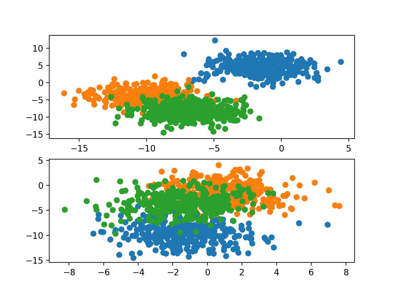
Running the example generates a sample of 1,000 examples for Problem 1 and Problem 2 and creates a scatter plot for each sample, coloring the data points by their class value.
Scatter Plots of Blobs Dataset for Problems 1 and 2 With Three Classes and Points Colored by Class Value
This provides a good basis for transfer learning as each version of the problem has similar input data with a similar scale, although with different target information (e.g. cluster centers).
We would expect that aspects of a model fit on one version of the blobs problem (e.g. Problem 1) to be useful when fitting a model on a new version of the blobs problem (e.g. Problem 2).
Multilayer Perceptron Model for Problem 1
In this section, we will develop a Multilayer Perceptron model (MLP) for Problem 1 and save the model to file so that we can reuse the weights later.
First, we will develop a function to prepare the dataset ready for modeling. After the make_blobs() function is called with a given random seed (e.g, one in this case for Problem 1), the target variable must be one hot encoded so that we can develop a model that predicts the probability of a given sample belonging to each of the target classes.
The prepared samples can then be split in half, with 500 examples for both the train and test datasets. The samples_for_seed() function below implements this, preparing the dataset for a given random number seed and re-tuning the train and test sets split into input and output components.
1
2
3
4
5
6
7
8
9
10
11
# prepare a blobs examples with a given random seed
We can call this function to prepare a dataset for Problem 1 as follows.
1
2
# prepare data
trainX,trainy,testX,testy=samples_for_seed(1)
Next, we can define and fit a model on the training dataset.
The model will expect two inputs for the two variables in the data. The model will have two hidden layers with five nodes each and the rectified linear activation function. Two layers are probably not required for this function, although we’re interested in the model learning some deep structure that we can reuse across instances of this problem. The output layer has three nodes, one for each class in the target variable and the softmax activation function.
Given that the problem is a multi-class classification problem, the categorical cross-entropy loss function is minimized and the stochastic gradient descent with the default learning rate and no momentum is used to learn the problem.
The model is fit for 100 epochs on the training dataset and the test set is used as a validation dataset during training, evaluating the performance on both datasets at the end of each epoch so that we can plot learning curves.
The fit_model() function ties these elements together, taking the train and test datasets as arguments and returning the fit model and training history.
The history collected during training can be used to create line plots showing both the loss and classification accuracy for the model on the train and test sets over each training epoch, providing learning curves.
The summarize_model() function below implements this, taking the fit model, training history, and dataset as arguments and printing the model performance and creating a plot of model learning curves.
At the end of the run, we can save the model to file so that we may load it later and use it as the basis for some transfer learning experiments.
Note that saving the model to file requires that you have the h5py library installed. This library can be installed via pip as follows:
1
sudo pip install h5py
The fit model can be saved by calling the save() function on the model.
1
2
# save model to file
model.save('model.h5')
Tying these elements together, the complete example of fitting an MLP on Problem 1, summarizing the model’s performance, and saving the model to file is listed below.
1
2
3
4
5
6
7
8
9
10
11
12
13
14
15
16
17
18
19
20
21
22
23
24
25
26
27
28
29
30
31
32
33
34
35
36
37
38
39
40
41
42
43
44
45
46
47
48
49
50
51
52
53
54
55
56
57
58
59
60
61
# fit mlp model on problem 1 and save model to file
from sklearn.datasets import make_blobs
from keras.layers import Dense
from keras.models import Sequential
from keras.optimizers import SGD
from keras.utils import to_categorical
from matplotlib import pyplot
# prepare a blobs examples with a given random seed
Running the example fits and evaluates the performance of the model, printing the classification accuracy on the train and test sets.
Note: Your results may vary given the stochastic nature of the algorithm or evaluation procedure, or differences in numerical precision. Consider running the example a few times and compare the average outcome.
In this case, we can see that the model performed well on Problem 1, achieving a classification accuracy of about 92% on both the train and test datasets.
1
Train: 0.916, Test: 0.920
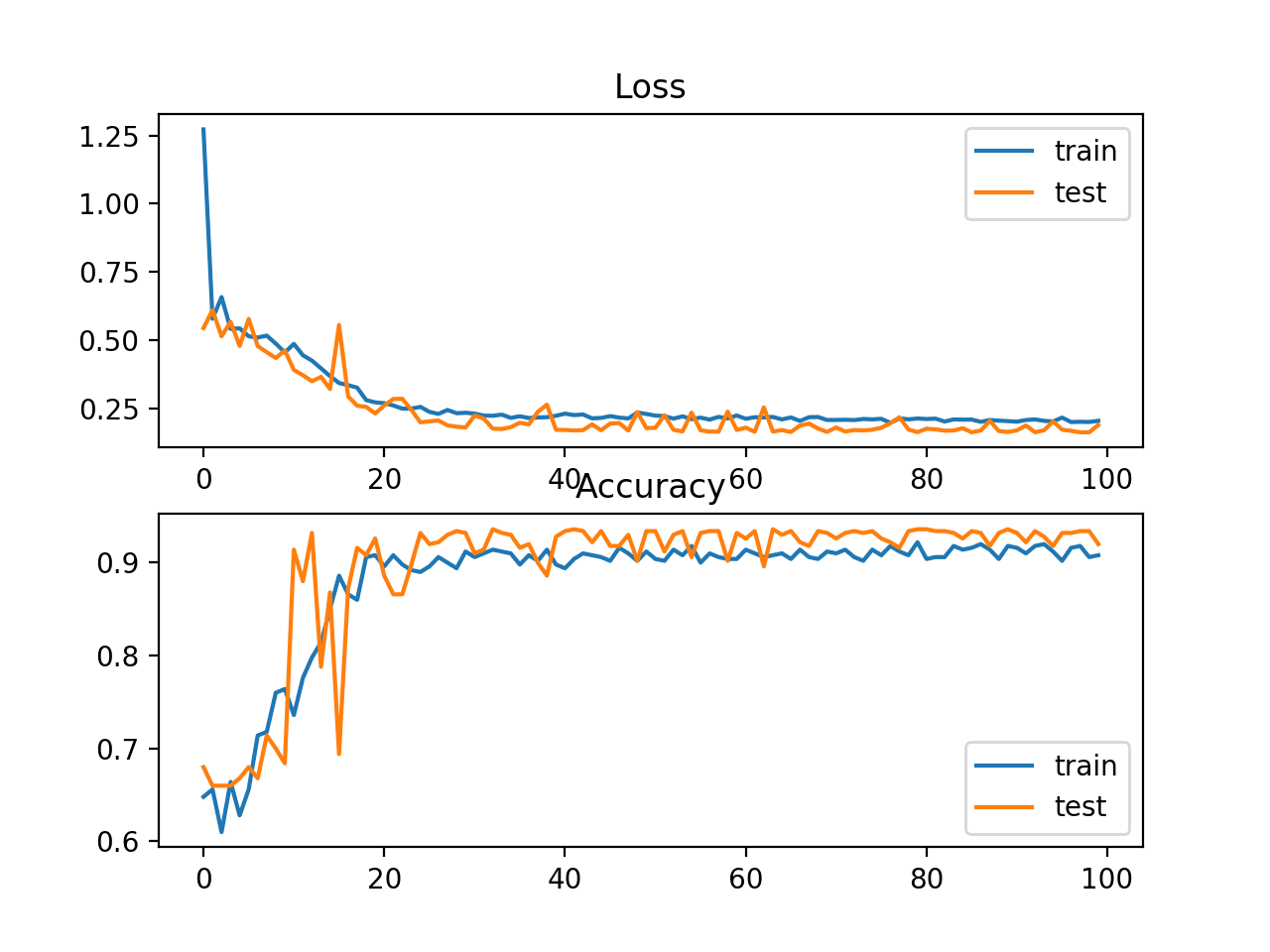
A figure is also created summarizing the learning curves of the model, showing both the loss (top) and accuracy (bottom) for the model on both the train (blue) and test (orange) datasets at the end of each training epoch.
Your plot may not look identical but is expected to show the same general behavior. If not, try running the example a few times.
In this case, we can see that the model learned the problem reasonably quickly and well, perhaps converging in about 40 epochs and remaining reasonably stable on both datasets.
Loss and Accuracy Learning Curves on the Train and Test Sets for an MLP on Problem 1
Now that we have seen how to develop a standalone MLP for the blobs Problem 1, we can look at the doing the same for Problem 2 that can be used as a baseline.
Standalone MLP Model for Problem 2
The example in the previous section can be updated to fit an MLP model to Problem 2.
It is important to get an idea of performance and learning dynamics on Problem 2 for a standalone model first as this will provide a baseline in performance that can be used to compare to a model fit on the same problem using transfer learning.
A single change is required that changes the call to samples_for_seed() to use the pseudorandom number generator seed of two instead of one.
1
2
# prepare data
trainX,trainy,testX,testy=samples_for_seed(2)
For completeness, the full example with this change is listed below.
1
2
3
4
5
6
7
8
9
10
11
12
13
14
15
16
17
18
19
20
21
22
23
24
25
26
27
28
29
30
31
32
33
34
35
36
37
38
39
40
41
42
43
44
45
46
47
48
49
50
51
52
53
54
55
56
57
58
59
# fit mlp model on problem 2 and save model to file
from sklearn.datasets import make_blobs
from keras.layers import Dense
from keras.models import Sequential
from keras.optimizers import SGD
from keras.utils import to_categorical
from matplotlib import pyplot
# prepare a blobs examples with a given random seed
Running the example fits and evaluates the performance of the model, printing the classification accuracy on the train and test sets.
Note: Your results may vary given the stochastic nature of the algorithm or evaluation procedure, or differences in numerical precision. Consider running the example a few times and compare the average outcome.
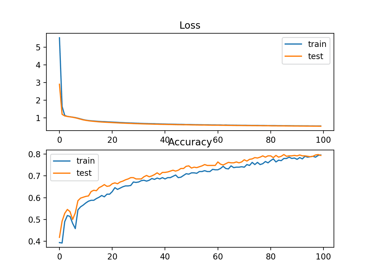
In this case, we can see that the model performed okay on Problem 2, but not as well as was seen on Problem 1, achieving a classification accuracy of about 79% on both the train and test datasets.
1
Train: 0.794, Test: 0.794
A figure is also created summarizing the learning curves of the model. Your plot may not look identical but is expected to show the same general behavior. If not, try running the example a few times.
In this case, we can see that the model converged more slowly than we saw on Problem 1 in the previous section. This suggests that this version of the problem may be slightly more challenging, at least for the chosen model configuration.
Loss and Accuracy Learning Curves on the Train and Test Sets for an MLP on Problem 2
Now that we have a baseline of performance and learning dynamics for an MLP on Problem 2, we can see how the addition of transfer learning affects the MLP on this problem.
MLP With Transfer Learning for Problem 2
The model that was fit on Problem 1 can be loaded and the weights can be used as the initial weights for a model fit on Problem 2.
This is a type of transfer learning where learning on a different but related problem is used as a type of weight initialization scheme.
This requires that the fit_model() function be updated to load the model and refit it on examples for Problem 2.
The model saved in ‘model.h5’ can be loaded using the load_model() Keras function.
1
2
# load model
model=load_model('model.h5')
Once loaded, the model can be compiled and fit as per normal.
The updated fit_model() with this change is listed below.
We would expect that a model that uses the weights from a model fit on a different but related problem to learn the problem perhaps faster in terms of the learning curve and perhaps result in lower generalization error, although these aspects would be dependent on the choice of problems and model.
For completeness, the full example with this change is listed below.
1
2
3
4
5
6
7
8
9
10
11
12
13
14
15
16
17
18
19
20
21
22
23
24
25
26
27
28
29
30
31
32
33
34
35
36
37
38
39
40
41
42
43
44
45
46
47
48
49
50
51
52
53
54
55
56
57
# transfer learning with mlp model on problem 2
from sklearn.datasets import make_blobs
from keras.layers import Dense
from keras.models import Sequential
from keras.optimizers import SGD
from keras.utils import to_categorical
from keras.models import load_model
from matplotlib import pyplot
# prepare a blobs examples with a given random seed
Running the example fits and evaluates the performance of the model, printing the classification accuracy on the train and test sets.
Note: Your results may vary given the stochastic nature of the algorithm or evaluation procedure, or differences in numerical precision. Consider running the example a few times and compare the average outcome.
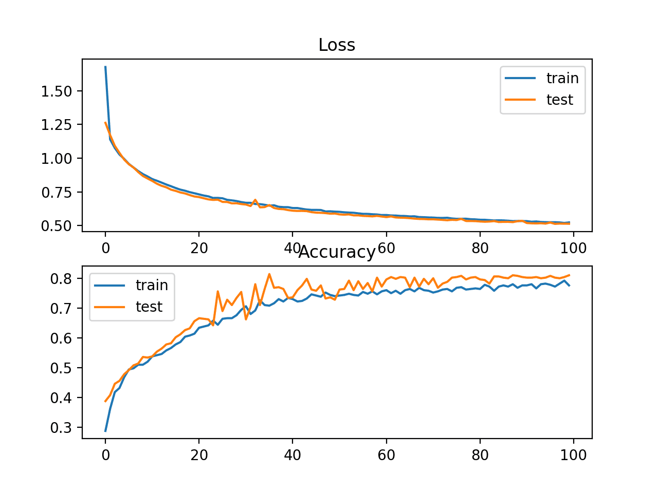
In this case, we can see that the model achieved a lower generalization error, achieving an accuracy of about 81% on the test dataset for Problem 2 as compared to the standalone model that achieved about 79% accuracy.
1
Train: 0.786, Test: 0.810
A figure is also created summarizing the learning curves of the model. Your plot may not look identical but is expected to show the same general behavior. If not, try running the example a few times.
In this case, we can see that the model does appear to have a similar learning curve, although we do see apparent improvements in the learning curve for the test set (orange line) both in terms of better performance earlier (epoch 20 onward) and above the performance of the model on the training set.
Loss and Accuracy Learning Curves on the Train and Test Sets for an MLP With Transfer Learning on Problem 2
We have only looked at single runs of a standalone MLP model and an MLP with transfer learning.
Neural network algorithms are stochastic, therefore an average of performance across multiple runs is required to see if the observed behavior is real or a statistical fluke.
Comparison of Models on Problem 2
In order to determine whether using transfer learning for the blobs multi-class classification problem has a real effect, we must repeat each experiment multiple times and analyze the average performance across the repeats.
We will compare the performance of the standalone model trained on Problem 2 to a model using transfer learning, averaged over 30 repeats.
Further, we will investigate whether keeping the weights in some of the layers fixed improves model performance.
The model trained on Problem 1 has two hidden layers. By keeping the first or the first and second hidden layers fixed, the layers with unchangeable weights will act as a feature extractor and may provide features that make learning Problem 2 easier, affecting the speed of learning and/or the accuracy of the model on the test set.
As the first step, we will simplify the fit_model() function to fit the model and discard any training history so that we can focus on the final accuracy of the trained model.
Next, we can develop a function that will repeatedly fit a new standalone model on Problem 2 on the training dataset and evaluate accuracy on the test set.
The eval_standalone_model() function below implements this, taking the train and test sets as arguments as well as the number of repeats and returns a list of accuracy scores for models on the test dataset.
Summarizing the distribution of accuracy scores returned from this function will give an idea of how well the chosen standalone model performs on Problem 2.
Next, we need an equivalent function for evaluating a model using transfer learning.
In each loop, the model trained on Problem 1 must be loaded from file, fit on the training dataset for Problem 2, then evaluated on the test set for Problem 2.
In addition, we will configure 0, 1, or 2 of the hidden layers in the loaded model to remain fixed. Keeping 0 hidden layers fixed means that all of the weights in the model will be adapted when learning Problem 2, using transfer learning as a weight initialization scheme. Whereas, keeping both (2) of the hidden layers fixed means that only the output layer of the model will be adapted during training, using transfer learning as a feature extraction method.
The eval_transfer_model() function below implements this, taking the train and test datasets for Problem 2 as arguments as well as the number of hidden layers in the loaded model to keep fixed and the number of times to repeat the experiment.
The function returns a list of test accuracy scores and summarizing this distribution will give a reasonable idea of how well the model with the chosen type of transfer learning performs on Problem 2.
1
2
3
4
5
6
7
8
9
10
11
12
13
14
15
16
17
# repeated evaluation of a model with transfer learning
In addition to reporting the mean and standard deviation of each model, we can collect all scores and create a box and whisker plot to summarize and compare the distributions of model scores.
Tying all of the these elements together, the complete example is listed below.
1
2
3
4
5
6
7
8
9
10
11
12
13
14
15
16
17
18
19
20
21
22
23
24
25
26
27
28
29
30
31
32
33
34
35
36
37
38
39
40
41
42
43
44
45
46
47
48
49
50
51
52
53
54
55
56
57
58
59
60
61
62
63
64
65
66
67
68
69
70
71
72
73
74
75
76
77
78
79
80
81
82
83
84
85
86
87
# compare standalone mlp model performance to transfer learning
from sklearn.datasets import make_blobs
from keras.layers import Dense
from keras.models import Sequential
from keras.optimizers import SGD
from keras.utils import to_categorical
from keras.models import load_model
from matplotlib import pyplot
from numpy import mean
from numpy import std
# prepare a blobs examples with a given random seed
Running the example first reports the mean and standard deviation of classification accuracy on the test dataset for each model.
Note: Your results may vary given the stochastic nature of the algorithm or evaluation procedure, or differences in numerical precision. Consider running the example a few times and compare the average outcome.
In this case, we can see that the standalone model achieved an accuracy of about 78% on Problem 2 with a large standard deviation of 10%. In contrast, we can see that the spread of all of the transfer learning models is much smaller, ranging from about 0.05% to 1.5%.
This difference in the standard deviations of the test accuracy scores shows the stability that transfer learning can bring to the model, reducing the variance in the performance of the final model introduced via the stochastic learning algorithm.
Comparing the mean test accuracy of the models, we can see that transfer learning that used the model as a weight initialization scheme (fixed=0) resulted in better performance than the standalone model with about 80% accuracy.
Keeping all hidden layers fixed (fixed=2) and using them as a feature extraction scheme resulted in worse performance on average than the standalone model. It suggests that the approach is too restrictive in this case.
Interestingly, we see best performance when the first hidden layer is kept fixed (fixed=1) and the second hidden layer is adapted to the problem with a test classification accuracy of about 81%. This suggests that in this case, the problem benefits from both the feature extraction and weight initialization properties of transfer learning.
It may be interesting to see how results of this last approach compare to the same model where the weights of the second hidden layer (and perhaps the output layer) are re-initialized with random numbers. This comparison would demonstrate whether the feature extraction properties of transfer learning alone or both feature extraction and weight initialization properties are beneficial.
1
2
3
4
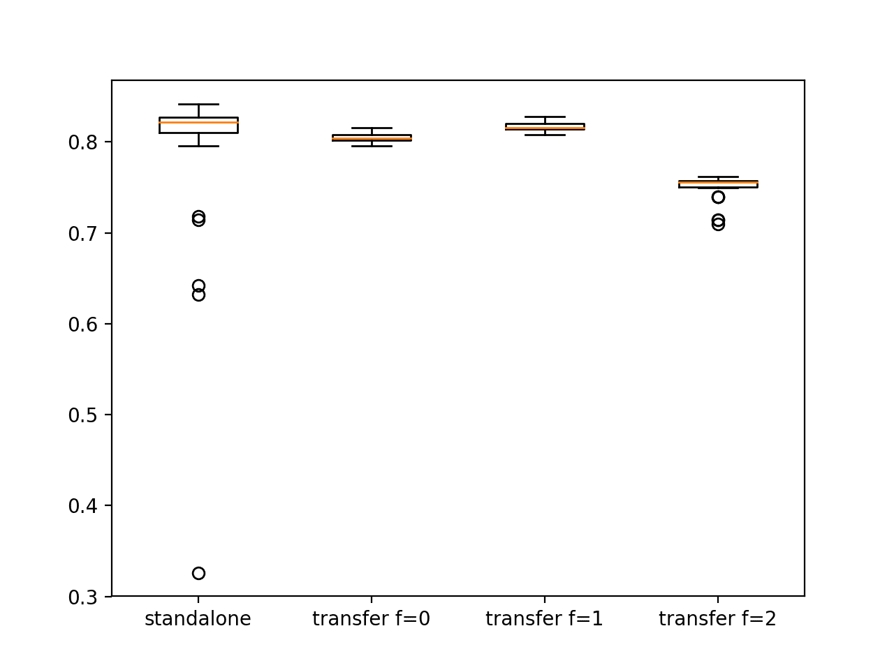
Standalone 0.787 (0.101)
Transfer (fixed=0) 0.805 (0.004)
Transfer (fixed=1) 0.817 (0.005)
Transfer (fixed=2) 0.750 (0.014)
A figure is created showing four box and whisker plots. The box shows the middle 50% of each data distribution, the orange line shows the median, and the dots show outliers.
The boxplot for the standalone model shows a number of outliers, indicating that on average, the model performs well, but there is a chance that it can perform very poorly.
Conversely, we see that the behavior of the models with transfer learning are more stable, showing a tighter distribution in performance.
Box and Whisker Plot Comparing Standalone and Transfer Learning Models via Test Set Accuracy on the Blobs Multiclass Classification Problem
Extensions
This section lists some ideas for extending the tutorial that you may wish to explore.
Reverse Experiment. Train and save a model for Problem 2 and see if it can help when using it for transfer learning on Problem 1.
Add Hidden Layer. Update the example to keep both hidden layers fixed, but add a new hidden layer with randomly initialized weights after the fixed layers before the output layer and compare performance.
Randomly Initialize Layers. Update the example to randomly initialize the weights of the second hidden layer and the output layer and compare performance.
If you explore any of these extensions, I’d love to know.
Further Reading
This section provides more resources on the topic if you are looking to go deeper.
Hi Jason,
Thanks for the tutorial.
1-Why do you have to (re-)compile the model used for transfer learning after loading? (The settings are the same)
2-Wouldn’t we expect a faster convergence rate for loss and accuracy using transfer learning? It does seem to be the case in your plots.
Hello Jason! Great tutorial. Could you explain a little bit further how you’ve come up with the box plots and outliers? I didn’t understand which data in particular leads to that representation (eg what is an outlier in this case) and how that data is generated. Thanks for your attention
Hello! Thank you for your answer. I’m sorry I didn’t make myself clear but I know what a box plot is. What I am trying to understand is what data is being plotted. How do we end up with several accuracies for each model?
Each model is evaluated multiple times. You are seeing the spread or variance of model performance given the stochastic nature of the learning algorithm and
Thank you for the tutorial, Jason!
By the way, I could not find “Section 5.2 Transfer Learning and Domain Adaptation, Deep Learning, 2016.” as your book reference but I can find the section at “15.2” not “5.2” Please check!
I read this post but still I have some questions. I am myself applying this transfer learning approach but can not move forward because of few doubts.
I have a trained multiclass text classification model consisting, Embedding, Bi-LSTM, output layer (Dense layer), now I want to add more data with more classes. My question is how to perform transfer learning in my case. I am freezing weights of Embedding layer and Bi LSTM layer but not of the output layer so its weights are randomly initialised. I dont’ achieve any good results. The accuracy looks good but the results are meaningless. I also coulld not find any good posts on Transfer learning in NLP, most of them are on Images using classifiers like Imagenet, Mobelnet etc.
Please give your suggestions, if you have any. Will appreciate your help.
Thank you!
Rishabh Sahrawat
Hi Jason, Again a great article. Can we apply transfer learning by adding new layer in trained model. If yes then How we can add ? Can you please help here.
When training dataset using transfer learning, loss & val_loss is reduced to about 25 and do not change any more. May I ask what’s the reason and how to solve it?
I always wondered why the pre-trained weights of a model constitute so large files! I mean at the end of the day they are just files with numbers corresponding to a large number of parameters! But why these pre-trained weight files are usually so large( >250 MB)?
splendid transfer learning tutorial!. Congratulations!
My questions:
1.) You mention fine-tuning on the tutorial intro. But it is not refer any more on the followings study cases.
To my understanding, any time you load the model weight coming from training problem 1, in order to solve problem 2, and allow to unfreeze some of the transfer model layers …you are performing some kind of fine-tuning “neurosurgery”. So you should mention it. Are you agree that you are performing fine-tuning even if you do not slow down the learning rate or apply other techniques?
2.) This not the case on your tutorial, but imagine you are training continually a model and saving your results in terms of trained weights.
Each time you get new or increase your (training) datasets …what would it be your strategy …to train the model with only the new “incremental” datasets but loading the previous trained model in a kind of fine-tuning (slow learning rate, using smooth SGD as optimizer, etc) BUT only applying only to the new incremental dataset or just to the whole training dataset or just training the whole dataset but starting from the scratch (I mean using random weights initialization e.g.) ?
which will be the best of the three strategies approach you would apply?
I read this post but still, I have some questions. I run your code on my computer directly but get a different result.
1. Multilayer Perceptron Model for Problem 1 :Train: 0.926, Test: 0.928
2. Standalone MLP Model for Problem 2 : Train: 0.808, Test: 0.812
3. MLP With Transfer Learning for Problem 2 : Train: 0.714, Test: 0.770
it seems like transfer learning is useless.
Appreciate this very helpful post.
My question is related to the model.fit( ) method. When trying to fit a pre trained model to new data, what is the difference between model.fit( ) and model.evaluate( ) ?
Doesn’t model.fit( ) just retrain the model on the new data instead of using weights from the old model?
Hi Jason,
Thanks a lot for the great tutorial,
I am trying to reproduce some results from a paper, which require using the weight reuse scheme you have described in the post but for a fully connected network with only one hidden layer which trained each time with different number of hidden units!! i have been trying to find a way to pass the wiegts to the larger network from the smaller one and initialze the extra hidden units randomly??
So my question is there a way to use transfer learning to a new network not with extra hidden
layer but with extra hidden units ??
Thanks a lot for your time and the great help we got from all of your posts
Changing the shape of the network would probably be invalid when reusing weights.
Unless you get creative and add additional nodes with random weights and some how freeze the nodes with pre-trained weights. Might require custom code.
Thank you so much for your great post. I have two questions:
1. May I use the model that is trained for a classification problem to be a pre-trained model for a regression problem using the transfer learning technique? If yes, how?
2. I trained several models and ensemble them together to become a new model. Can I use this new model as a pre-trained model to do transfer learning?
Keeping 0 hidden layers fixed means that all of the weights in the model will be adapted when learning Problem 2, using transfer learning as a weight initialization scheme.
Thanks for this interesting tutorial. My question is why do you think transfer learning works for this simple problem with a multi-layer perceptron model?
I kinda understand why transfer learning works on image tasks as lower convolutional layers learn basic image features and patterns, which would remain useful for any kind of image tasks. Therefore we can just retrain the final few layers or slap on a few more FC layers at the back to adapt to a specific task.
In this example, do you think transfer learning improves the result by acting as a kind of regularization?
The example here is just to help explain the idea of transfer learning. In general, deep learning has many layers of perceptrons. Usually the first few layers are to extract useful features from the input. If your input are of the similar type, we can expect the features are the same even the later layers will use them differently. This is why transfer learning helps.
hello dear dr jason. i have a problem about cnn accuracy. i have a multi class dataset with 10 classes which is about a retail site items. in every class there are a lot of different items based on a category e.g cameras,laptops,batteries are in class 1 …does this order of different things which have some common attributes
affect the problem? should i think about a special network or changing something about dataset.
i have tried many network..regularization techniques..data augmentation..but i couldnt reach to high validation accuracy…i had 2 sort of results:1) high training … low valid (overfitting) and 2) 50 – 50 accuracy and valid… i cant reach higher
accuracy. by the way thank you for this amazing site .. i have learned many thing of you .best regards.
Hi Sina…Thank you the feedback and kind words! While I cannot speak directly to your specific application, in general, if data is normalized and not considered “time-series” data, order should not be a major concern. If the data is staged as a time-series then is definitely important and you may even be able to benefit further by using Bi-Directional LSTMs.
hello again thanks for your reply…maybe i have use wrong words in my question.
the major thing is that in contrast to the other available datasets, there are multiple kind of items in every class of my dataset like i said before.
and also i think there is some noise too. e.g. some unrelated images between each class.
i’m trying to do image recognition with cnn then what is your suggestion to improve my
accuracy for valid data?
is it some way to manipulate this dataset?
by the way this dataset belongs to a company coompetition.
i have tried many things.. but i found out maybe the way that training dataset is being classifed is the problem.
Thank you for the tutorial
But can we apply transfer learning to a regression problem like
Earthquake Magnitude prediction if anyone has a model please help me.
A wonderful introduction to transfer learning. Thanks for your time and effort on this tutorial.
I have a question. Have you tried the transfer techniques mentioned in this post for regression tasks? Transfer learning is more common on image classification tasks and I couldn’t find much about transfer learning techniques for regression tasks.
As per your knowledge, how would the transfer learning fare for regression tasks?
Thank you for this amazing tutorial on transfer learning. I am new to it and working on a regression problem . In my case the input dimension is different from the base model and I m using ANN. Kindly guide me on this.
Thank you for this amazing tutorial on transfer learning. I am new to it and working on a regression problem . In my case the input dimension is different from the base model and I m using ANN. Kindly guide me on this.
Thank you so much for this amazing tutorial on transfer learning. Currently i m working on transfer learning on regression task. My problem is my input dimension is different from the base model. Can you please help me to solve this?
Thanks for the amazing explanation of yours. I just wanted to ask, the part where you freeze 0, 1 and 2 layers of the MLP, doesn’t your code select the first, second and third layer to freeze instead of freezing none, one and both layers to freeze?
Also, what would be the reason for having a little variance even when we freeze all layers? Freezing layers would mean there is no adaptation anymore so no weigh randomization, no SGD, so where does the variance come from?


Hi Jason,
Thanks for the tutorial.
1-Why do you have to (re-)compile the model used for transfer learning after loading? (The settings are the same)
2-Wouldn’t we expect a faster convergence rate for loss and accuracy using transfer learning? It does seem to be the case in your plots.
Keras prefers the model to be compiled before use, so that it can nail down the shapes of the transforms to be applied.
It depends on the type of problem, perhaps.
I also didn’t understand this, if you have to compile, and fit the previous model on the data again, how are you usig the previous weights?
Are you just using the previous weights as initialization weights for the second model?
Yes. The weights from the prior model can be used as-is and frozen (not changed) or used as a starting point. We explore both approaches.
Hello Jason! Great tutorial. Could you explain a little bit further how you’ve come up with the box plots and outliers? I didn’t understand which data in particular leads to that representation (eg what is an outlier in this case) and how that data is generated. Thanks for your attention
Yes, the data is plotted using a boxplot:
https://matplotlib.org/3.1.1/api/_as_gen/matplotlib.pyplot.boxplot.html
For more on how boxplots work:
https://en.wikipedia.org/wiki/Box_plot
Hello! Thank you for your answer. I’m sorry I didn’t make myself clear but I know what a box plot is. What I am trying to understand is what data is being plotted. How do we end up with several accuracies for each model?
Each model is evaluated multiple times. You are seeing the spread or variance of model performance given the stochastic nature of the learning algorithm and
Thank you for the tutorial, Jason!
By the way, I could not find “Section 5.2 Transfer Learning and Domain Adaptation, Deep Learning, 2016.” as your book reference but I can find the section at “15.2” not “5.2” Please check!
Yes, that was a typo, thanks, fixed!
Hi Dr. Brownlee,
I read this post but still I have some questions. I am myself applying this transfer learning approach but can not move forward because of few doubts.
I have a trained multiclass text classification model consisting, Embedding, Bi-LSTM, output layer (Dense layer), now I want to add more data with more classes. My question is how to perform transfer learning in my case. I am freezing weights of Embedding layer and Bi LSTM layer but not of the output layer so its weights are randomly initialised. I dont’ achieve any good results. The accuracy looks good but the results are meaningless. I also coulld not find any good posts on Transfer learning in NLP, most of them are on Images using classifiers like Imagenet, Mobelnet etc.
Please give your suggestions, if you have any. Will appreciate your help.
Thank you!
Rishabh Sahrawat
Perhaps fit the model on one dataset, then transfer to new dataset and use a very small learning rate to tune the model to the new data?
Hi Jason, Again a great article. Can we apply transfer learning by adding new layer in trained model. If yes then How we can add ? Can you please help here.
Thank you !!
Yes. You can use the Keras functional API to add new layers to existing models.
When training dataset using transfer learning, loss & val_loss is reduced to about 25 and do not change any more. May I ask what’s the reason and how to solve it?
Yes, the tutorials here will help you diagnose the learning dynamics and give techniques to improve the learning:
https://machinelearningmastery.com/start-here/#better
Hello,
I always wondered why the pre-trained weights of a model constitute so large files! I mean at the end of the day they are just files with numbers corresponding to a large number of parameters! But why these pre-trained weight files are usually so large( >250 MB)?
Cheers!
Good question.
Perhaps there are simply lots of 64-bit numbers.
Hi Jason:
splendid transfer learning tutorial!. Congratulations!
My questions:
1.) You mention fine-tuning on the tutorial intro. But it is not refer any more on the followings study cases.
To my understanding, any time you load the model weight coming from training problem 1, in order to solve problem 2, and allow to unfreeze some of the transfer model layers …you are performing some kind of fine-tuning “neurosurgery”. So you should mention it. Are you agree that you are performing fine-tuning even if you do not slow down the learning rate or apply other techniques?
2.) This not the case on your tutorial, but imagine you are training continually a model and saving your results in terms of trained weights.
Each time you get new or increase your (training) datasets …what would it be your strategy …to train the model with only the new “incremental” datasets but loading the previous trained model in a kind of fine-tuning (slow learning rate, using smooth SGD as optimizer, etc) BUT only applying only to the new incremental dataset or just to the whole training dataset or just training the whole dataset but starting from the scratch (I mean using random weights initialization e.g.) ?
which will be the best of the three strategies approach you would apply?
thank you very much for your valuable lessons!
Thanks.
Yes, although “fine tuning” often has a specific meaning – training pre-trained weights on more data and using a very small learning rate.
Rather than guess, I would use controlled experiments to discover the best update strategy for the data/domain.
Dear Jason,
thank you for the effort you put into the essay.
I am wondering about whether fin tuning has the same mining as weight initialization?
I cannot understand the difference between fine-tuning, weight initialization?
Thank you for your answer.
Fining tuning changes the model weights for a new data, performed after transfer learning.
Weight initializing sets the weights to small random values prior to training a model.
Hi Dr Brownlee,
I read this post but still, I have some questions. I run your code on my computer directly but get a different result.
1. Multilayer Perceptron Model for Problem 1 :Train: 0.926, Test: 0.928
2. Standalone MLP Model for Problem 2 : Train: 0.808, Test: 0.812
3. MLP With Transfer Learning for Problem 2 : Train: 0.714, Test: 0.770
it seems like transfer learning is useless.
Here we are showing how to do transfer learning, the specific application is just a context to understand the method.
Hi Jason,
Appreciate this very helpful post.
My question is related to the model.fit( ) method. When trying to fit a pre trained model to new data, what is the difference between model.fit( ) and model.evaluate( ) ?
Doesn’t model.fit( ) just retrain the model on the new data instead of using weights from the old model?
Appreciate your response on this. Thanks.
fit() will train the model.
evaluate() will use the model to make predictions and calculate the error on those predictions.
Hi Jason,
Thanks a lot for the great tutorial,
I am trying to reproduce some results from a paper, which require using the weight reuse scheme you have described in the post but for a fully connected network with only one hidden layer which trained each time with different number of hidden units!! i have been trying to find a way to pass the wiegts to the larger network from the smaller one and initialze the extra hidden units randomly??
So my question is there a way to use transfer learning to a new network not with extra hidden
layer but with extra hidden units ??
Thanks a lot for your time and the great help we got from all of your posts
Changing the shape of the network would probably be invalid when reusing weights.
Unless you get creative and add additional nodes with random weights and some how freeze the nodes with pre-trained weights. Might require custom code.
Thank you so much for your great post. I have two questions:
1. May I use the model that is trained for a classification problem to be a pre-trained model for a regression problem using the transfer learning technique? If yes, how?
2. I trained several models and ensemble them together to become a new model. Can I use this new model as a pre-trained model to do transfer learning?
Many thanks
You’re welcome!
Yes. Save the model, load the model, train some or all layers on new data. The above tutorial will get you started directly with this.
Yes, you can use an ensemble of models in transfer learning if you like.
Hi Jason,
In your code, fixed = 0 actually means that you fixed the first layer since the index starts from 0.
So, when fixed = 0 you have basically locked the first layer of your neural network. Am I correct?
Yes, 0 is the first hidden layer. Not the input layer.
So, fixed = 0 is also under the feature extraction scheme not the weight initialization scheme. Right?
Not really, fixed=0 means all weights are updated.
Fixed = 0 means that all the weights in the first hidden layer are fixed. The weights in the rest of the hidden layers are updated. Right?
From the tutorial:
Hi Jason,
Thanks for this interesting tutorial. My question is why do you think transfer learning works for this simple problem with a multi-layer perceptron model?
I kinda understand why transfer learning works on image tasks as lower convolutional layers learn basic image features and patterns, which would remain useful for any kind of image tasks. Therefore we can just retrain the final few layers or slap on a few more FC layers at the back to adapt to a specific task.
In this example, do you think transfer learning improves the result by acting as a kind of regularization?
The example here is just to help explain the idea of transfer learning. In general, deep learning has many layers of perceptrons. Usually the first few layers are to extract useful features from the input. If your input are of the similar type, we can expect the features are the same even the later layers will use them differently. This is why transfer learning helps.
hello dear dr jason. i have a problem about cnn accuracy. i have a multi class dataset with 10 classes which is about a retail site items. in every class there are a lot of different items based on a category e.g cameras,laptops,batteries are in class 1 …does this order of different things which have some common attributes
affect the problem? should i think about a special network or changing something about dataset.
i have tried many network..regularization techniques..data augmentation..but i couldnt reach to high validation accuracy…i had 2 sort of results:1) high training … low valid (overfitting) and 2) 50 – 50 accuracy and valid… i cant reach higher
accuracy. by the way thank you for this amazing site .. i have learned many thing of you .best regards.
Hi Sina…Thank you the feedback and kind words! While I cannot speak directly to your specific application, in general, if data is normalized and not considered “time-series” data, order should not be a major concern. If the data is staged as a time-series then is definitely important and you may even be able to benefit further by using Bi-Directional LSTMs.
https://machinelearningmastery.com/develop-bidirectional-lstm-sequence-classification-python-keras/
hello again thanks for your reply…maybe i have use wrong words in my question.
the major thing is that in contrast to the other available datasets, there are multiple kind of items in every class of my dataset like i said before.
and also i think there is some noise too. e.g. some unrelated images between each class.
i’m trying to do image recognition with cnn then what is your suggestion to improve my
accuracy for valid data?
is it some way to manipulate this dataset?
by the way this dataset belongs to a company coompetition.
i have tried many things.. but i found out maybe the way that training dataset is being classifed is the problem.
Thank you for the tutorial
But can we apply transfer learning to a regression problem like
Earthquake Magnitude prediction if anyone has a model please help me.
Hi Ewnetu…the following resource may be of interest to you:
https://link.springer.com/chapter/10.1007/978-3-030-66763-4_4
Hello James,
A wonderful introduction to transfer learning. Thanks for your time and effort on this tutorial.
I have a question. Have you tried the transfer techniques mentioned in this post for regression tasks? Transfer learning is more common on image classification tasks and I couldn’t find much about transfer learning techniques for regression tasks.
As per your knowledge, how would the transfer learning fare for regression tasks?
Thanks!
Hi Sandesh…You are very welcome! This is a great question and you are correct that most references consider classification.
The following resources may be of interest:
https://arxiv.org/abs/2102.09504
https://www.quora.com/Can-transfer-learning-be-applied-for-regression-tasks-and-are-there-other-ways-of-using-transfer-learning-other-than-through-neural-networks
Hello James,
Thank you for this amazing tutorial on transfer learning. I am new to it and working on a regression problem . In my case the input dimension is different from the base model and I m using ANN. Kindly guide me on this.
Hello James,
Thank you for this amazing tutorial on transfer learning. I am new to it and working on a regression problem . In my case the input dimension is different from the base model and I m using ANN. Kindly guide me on this.
Hello Dr. Brownlee,
Thank you so much for this amazing tutorial on transfer learning. Currently i m working on transfer learning on regression task. My problem is my input dimension is different from the base model. Can you please help me to solve this?
Hi Shaggy…You are very welcome! The following resource is a great starting points for application of transfer learning:
https://machinelearningmastery.com/transfer-learning-for-deep-learning/
Hey Jason,
Thanks for the amazing explanation of yours. I just wanted to ask, the part where you freeze 0, 1 and 2 layers of the MLP, doesn’t your code select the first, second and third layer to freeze instead of freezing none, one and both layers to freeze?
Also, what would be the reason for having a little variance even when we freeze all layers? Freezing layers would mean there is no adaptation anymore so no weigh randomization, no SGD, so where does the variance come from?
Thanks a lot
Hi Apollonia…You are very welcome! The following resource may be of interest to you.
https://analyticsindiamag.com/what-does-freezing-a-layer-mean-and-how-does-it-help-in-fine-tuning-neural-networks/