The Pix2Pix GAN is a generator model for performing image-to-image translation trained on paired examples.
For example, the model can be used to translate images of daytime to nighttime, or from sketches of products like shoes to photographs of products.
The benefit of the Pix2Pix model is that compared to other GANs for conditional image generation, it is relatively simple and capable of generating large high-quality images across a variety of image translation tasks.
The model is very impressive but has an architecture that appears somewhat complicated to implement for beginners.
In this tutorial, you will discover how to implement the Pix2Pix GAN architecture from scratch using the Keras deep learning framework.
After completing this tutorial, you will know:
How to develop the PatchGAN discriminator model for the Pix2Pix GAN.
How to develop the U-Net encoder-decoder generator model for the Pix2Pix GAN.
How to implement the composite model for updating the generator and how to train both models.
The GAN architecture is comprised of a generator model for outputting new plausible synthetic images and a discriminator model that classifies images as real (from the dataset) or fake (generated). The discriminator model is updated directly, whereas the generator model is updated via the discriminator model. As such, the two models are trained simultaneously in an adversarial process where the generator seeks to better fool the discriminator and the discriminator seeks to better identify the counterfeit images.
The Pix2Pix model is a type of conditional GAN, or cGAN, where the generation of the output image is conditional on an input, in this case, a source image. The discriminator is provided both with a source image and the target image and must determine whether the target is a plausible transformation of the source image.
Again, the discriminator model is updated directly, and the generator model is updated via the discriminator model, although the loss function is updated. The generator is trained via adversarial loss, which encourages the generator to generate plausible images in the target domain. The generator is also updated via L1 loss measured between the generated image and the expected output image. This additional loss encourages the generator model to create plausible translations of the source image.
The Pix2Pix GAN has been demonstrated on a range of image-to-image translation tasks such as converting maps to satellite photographs, black and white photographs to color, and sketches of products to product photographs.
Now that we are familiar with the Pix2Pix GAN, let’s explore how we can implement it using the Keras deep learning library.
Want to Develop GANs from Scratch?
Take my free 7-day email crash course now (with sample code).
Click to sign-up and also get a free PDF Ebook version of the course.
How to Implement the PatchGAN Discriminator Model
The discriminator model in the Pix2Pix GAN is implemented as a PatchGAN.
The PatchGAN is designed based on the size of the receptive field, sometimes called the effective receptive field. The receptive field is the relationship between one output activation of the model to an area on the input image (actually volume as it proceeded down the input channels).
A PatchGAN with the size 70×70 is used, which means that the output (or each output) of the model maps to a 70×70 square of the input image. In effect, a 70×70 PatchGAN will classify 70×70 patches of the input image as real or fake.
… we design a discriminator architecture – which we term a PatchGAN – that only penalizes structure at the scale of patches. This discriminator tries to classify if each NxN patch in an image is real or fake. We run this discriminator convolutionally across the image, averaging all responses to provide the ultimate output of D.
Before we dive into the configuration details of the PatchGAN, it is important to get a handle on the calculation of the receptive field.
The receptive field is not the size of the output of the discriminator model, e.g. it does not refer to the shape of the activation map output by the model. It is a definition of the model in terms of one pixel in the output activation map to the input image. The output of the model may be a single value or a square activation map of values that predict whether each patch of the input image is real or fake.
Traditionally, the receptive field refers to the size of the activation map of a single convolutional layer with regards to the input of the layer, the size of the filter, and the size of the stride. The effective receptive field generalizes this idea and calculates the receptive field for the output of a stack of convolutional layers with regard to the raw image input. The terms are often used interchangeably.
The authors of the Pix2Pix GAN provide a Matlab script to calculate the effective receptive field size for different model configurations in a script called receptive_field_sizes.m. It can be helpful to work through an example for the 70×70 PatchGAN receptive field calculation.
The 70×70 PatchGAN has a fixed number of three layers (excluding the output and second last layers), regardless of the size of the input image. The calculation of the receptive field in one dimension is calculated as:
Where output size is the size of the prior layers activation map, stride is the number of pixels the filter is moved when applied to the activation, and kernel size is the size of the filter to be applied.
The PatchGAN uses a fixed stride of 2×2 (except in the output and second last layers) and a fixed kernel size of 4×4. We can, therefore, calculate the receptive field size starting with one pixel in the output of the model and working backward to the input image.
We can develop a Python function called receptive_field() to calculate the receptive field, then calculate and print the receptive field for each layer in the Pix2Pix PatchGAN model. The complete example is listed below.
1
2
3
4
5
6
7
8
9
10
11
12
13
14
15
16
17
18
19
# example of calculating the receptive field for the PatchGAN
# output layer 1x1 pixel with 4x4 kernel and 1x1 stride
rf=receptive_field(1,4,1)
print(rf)
# second last layer with 4x4 kernel and 1x1 stride
rf=receptive_field(rf,4,1)
print(rf)
# 3 PatchGAN layers with 4x4 kernel and 2x2 stride
rf=receptive_field(rf,4,2)
print(rf)
rf=receptive_field(rf,4,2)
print(rf)
rf=receptive_field(rf,4,2)
print(rf)
Running the example prints the size of the receptive field for each layer in the model from the output layer to the input layer.
We can see that each 1×1 pixel in the output layer maps to a 70×70 receptive field in the input layer.
1
2
3
4
5
4
7
16
34
70
The authors of the Pix2Pix paper explore different PatchGAN configurations, including a 1×1 receptive field called a PixelGAN and a receptive field that matches the 256×256 pixel images input to the model (resampled to 286×286) called an ImageGAN. They found that the 70×70 PatchGAN resulted in the best trade-off of performance and image quality.
The 70×70 PatchGAN […] achieves slightly better scores. Scaling beyond this, to the full 286×286 ImageGAN, does not appear to improve the visual quality of the results.
The model takes two images as input, specifically a source and a target image. These images are concatenated together at the channel level, e.g. 3 color channels of each image become 6 channels of the input.
Let Ck denote a Convolution-BatchNorm-ReLU layer with k filters. […] All convolutions are 4× 4 spatial filters applied with stride 2. […] The 70 × 70 discriminator architecture is: C64-C128-C256-C512. After the last layer, a convolution is applied to map to a 1-dimensional output, followed by a Sigmoid function. As an exception to the above notation, BatchNorm is not applied to the first C64 layer. All ReLUs are leaky, with slope 0.2.
The PatchGAN configuration is defined using a shorthand notation as: C64-C128-C256-C512, where C refers to a block of Convolution-BatchNorm-LeakyReLU layers and the number indicates the number of filters. Batch normalization is not used in the first layer. As mentioned, the kernel size is fixed at 4×4 and a stride of 2×2 is used on all but the last 2 layers of the model. The slope of the LeakyReLU is set to 0.2, and a sigmoid activation function is used in the output layer.
Random jitter was applied by resizing the 256×256 input images to 286 × 286 and then randomly cropping back to size 256 × 256. Weights were initialized from a Gaussian distribution with mean 0 and standard deviation 0.02.
Model weights were initialized via random Gaussian with a mean of 0.0 and standard deviation of 0.02. Images input to the model are 256×256.
… we divide the objective by 2 while optimizing D, which slows down the rate at which D learns relative to G. We use minibatch SGD and apply the Adam solver, with a learning rate of 0.0002, and momentum parameters β1 = 0.5, β2 = 0.999.
The model is trained with a batch size of one image and the Adam version of stochastic gradient descent is used with a small learning range and modest momentum. The loss for the discriminator is weighted by 50% for each model update.
Tying this all together, we can define a function named define_discriminator() that creates the 70×70 PatchGAN discriminator model.
The complete example of defining the model is listed below.
1
2
3
4
5
6
7
8
9
10
11
12
13
14
15
16
17
18
19
20
21
22
23
24
25
26
27
28
29
30
31
32
33
34
35
36
37
38
39
40
41
42
43
44
45
46
47
48
49
50
51
52
53
54
55
56
57
58
59
# example of defining a 70x70 patchgan discriminator model
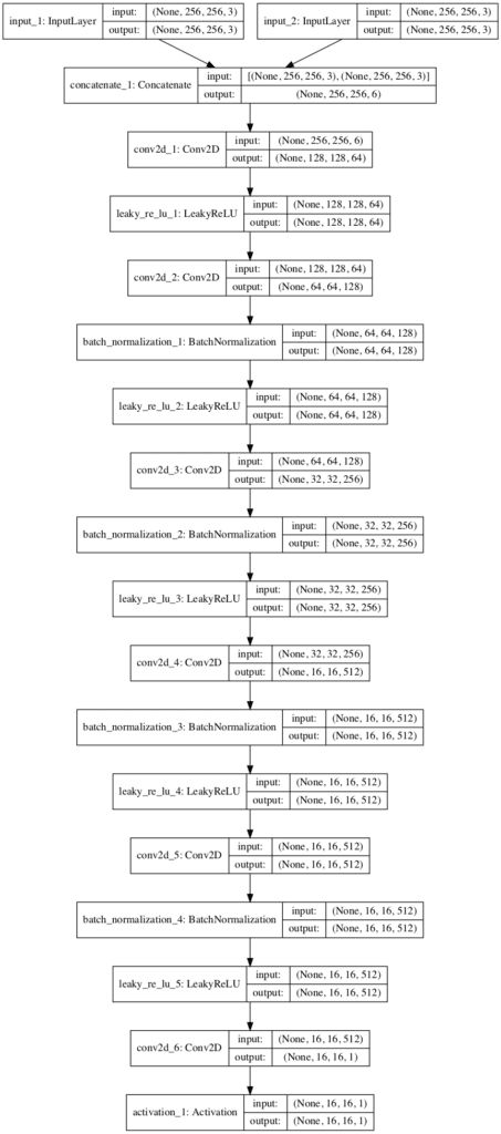
Running the example first summarizes the model, providing insight into how the input shape is transformed across the layers and the number of parameters in the model.
We can see that the two input images are concatenated together to create one 256x256x6 input to the first hidden convolutional layer. This concatenation of input images could occur before the input layer of the model, but allowing the model to perform the concatenation makes the behavior of the model clearer.
We can see that the model output will be an activation map with the size 16×16 pixels or activations and a single channel, with each value in the map corresponding to a 70×70 pixel patch of the input 256×256 image. If the input image was half the size at 128×128, then the output feature map would also be halved to 8×8.
The model is a binary classification model, meaning it predicts an output as a probability in the range [0,1], in this case, the likelihood of whether the input image is real or from the target dataset. The patch of values can be averaged to give a real/fake prediction by the model. When trained, the target is compared to a matrix of target values, 0 for fake and 1 for real.
A plot of the model is created showing much the same information in a graphical form. The model is not complex, with a linear path with two input images and a single output prediction.
Note: creating the plot assumes that pydot and pygraphviz libraries are installed. If this is a problem, you can comment out the import and call to the plot_model() function.
Plot of the PatchGAN Model Used in the Pix2Pix GAN Architecture
Now that we know how to implement the PatchGAN discriminator model, we can now look at implementing the U-Net generator model.
How to Implement the U-Net Generator Model
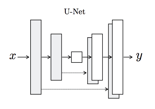
The generator model for the Pix2Pix GAN is implemented as a U-Net.
The U-Net model is an encoder-decoder model for image translation where skip connections are used to connect layers in the encoder with corresponding layers in the decoder that have the same sized feature maps.
The encoder part of the model is comprised of convolutional layers that use a 2×2 stride to downsample the input source image down to a bottleneck layer. The decoder part of the model reads the bottleneck output and uses transpose convolutional layers to upsample to the required output image size.
… the input is passed through a series of layers that progressively downsample, until a bottleneck layer, at which point the process is reversed.
Architecture of the U-Net Generator Model Taken from Image-to-Image Translation With Conditional Adversarial Networks.
Skip connections are added between the layers with the same sized feature maps so that the first downsampling layer is connected with the last upsampling layer, the second downsampling layer is connected with the second last upsampling layer, and so on. The connections concatenate the channels of the feature map in the downsampling layer with the feature map in the upsampling layer.
Specifically, we add skip connections between each layer i and layer n − i, where n is the total number of layers. Each skip connection simply concatenates all channels at layer i with those at layer n − i.
Unlike traditional generator models in the GAN architecture, the U-Net generator does not take a point from the latent space as input. Instead, dropout layers are used as a source of randomness both during training and when the model is used to make a prediction, e.g. generate an image at inference time.
Similarly, batch normalization is used in the same way during training and inference, meaning that statistics are calculated for each batch and not fixed at the end of the training process. This is referred to as instance normalization, specifically when the batch size is set to 1 as it is with the Pix2Pix model.
At inference time, we run the generator net in exactly the same manner as during the training phase. This differs from the usual protocol in that we apply dropout at test time, and we apply batch normalization using the statistics of the test batch, rather than aggregated statistics of the training batch.
In Keras, layers like Dropout and BatchNormalization operate differently during training and in inference model. We can set the “training” argument when calling these layers to “True” to ensure that they always operate in training-model, even when used during inference.
For example, a Dropout layer that will drop out during inference as well as training can be added to the model as follows:
The encoder uses blocks of Convolution-BatchNorm-LeakyReLU like the discriminator model, whereas the decoder model uses blocks of Convolution-BatchNorm-Dropout-ReLU with a dropout rate of 50%. All convolutional layers use a filter size of 4×4 and a stride of 2×2.
Let Ck denote a Convolution-BatchNorm-ReLU layer with k filters. CDk denotes a Convolution-BatchNormDropout-ReLU layer with a dropout rate of 50%. All convolutions are 4× 4 spatial filters applied with stride 2.
The last layer of the encoder is the bottleneck layer, which does not use batch normalization, according to an amendment to the paper and confirmation in the code, and uses a ReLU activation instead of LeakyRelu.
… the activations of the bottleneck layer are zeroed by the batchnorm operation, effectively making the innermost layer skipped. This issue can be fixed by removing batchnorm from this layer, as has been done in the public code
The number of filters in the U-Net decoder is a little misleading as it is the number of filters for the layer after concatenation with the equivalent layer in the encoder. This may become more clear when we create a plot of the model.
The output of the model uses a single convolutional layer with three channels, and tanh activation function is used in the output layer, common to GAN generator models. Batch normalization is not used in the first layer of the encoder.
After the last layer in the decoder, a convolution is applied to map to the number of output channels (3 in general […]), followed by a Tanh function […] BatchNorm is not applied to the first C64 layer in the encoder. All ReLUs in the encoder are leaky, with slope 0.2, while ReLUs in the decoder are not leaky.
Tying this all together, we can define a function named define_generator() that defines the U-Net encoder-decoder generator model. Two helper functions are also provided for defining encoder blocks of layers and decoder blocks of layers.
The complete example of defining the model is listed below.
1
2
3
4
5
6
7
8
9
10
11
12
13
14
15
16
17
18
19
20
21
22
23
24
25
26
27
28
29
30
31
32
33
34
35
36
37
38
39
40
41
42
43
44
45
46
47
48
49
50
51
52
53
54
55
56
57
58
59
60
61
62
63
64
65
66
67
68
69
70
71
72
73
74
75
76
77
78
79
80
81
82
83
84
# example of defining a u-net encoder-decoder generator model
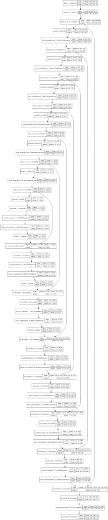
A plot of the model is created showing much the same information in a graphical form. The model is complex, and the plot helps to understand the skip connections and their impact on the number of filters in the decoder.
Note: creating the plot assumes that pydot and pygraphviz libraries are installed. If this is a problem, you can comment out the import and call to the plot_model() function.
Working backward from the output layer, if we look at the Concatenate layers and the first Conv2DTranspose layer of the decoder, we can see the number of channels as:
[128, 256, 512, 1024, 1024, 1024, 1024, 512].
Reversing this list gives the stated configuration of the number of filters for each layer in the decoder from the paper of:
CD512-CD1024-CD1024-C1024-C1024-C512-C256-C128
Plot of the U-Net Encoder-Decoder Model Used in the Pix2Pix GAN Architecture
Now that we have defined both models, we can look at how the generator model is updated via the discriminator model.
How to Implement Adversarial and L1 Loss
The discriminator model can be updated directly, whereas the generator model must be updated via the discriminator model.
This can be achieved by defining a new composite model in Keras that connects the output of the generator model as input to the discriminator model. The discriminator model can then predict whether a generated image is real or fake. We can update the weights of the composite model in such a way that the generated image has the label of “real” instead of “fake“, which will cause the generator weights to be updated towards generating a better fake image. We can also mark the discriminator weights as not trainable in this context, to avoid the misleading update.
Additionally, the generator needs to be updated to better match the targeted translation of the input image. This means that the composite model must also output the generated image directly, allowing it to be compared to the target image.
Therefore, we can summarize the inputs and outputs of this composite model as follows:
Inputs: Source image
Outputs: Classification of real/fake, generated target image.
The weights of the generator will be updated via both adversarial loss via the discriminator output and L1 loss via the direct image output. The loss scores are added together, where the L1 loss is treated as a regularizing term and weighted via a hyperparameter called lambda, set to 100.
loss = adversarial loss + lambda * L1 loss
The define_gan() function below implements this, taking the defined generator and discriminator models as input and creating the composite GAN model that can be used to update the generator model weights.
The source image input is provided both to the generator and the discriminator as input and the output of the generator is also connected to the discriminator as input.
Two loss functions are specified when the model is compiled for the discriminator and generator outputs respectively. The loss_weights argument is used to define the weighting of each loss when added together to update the generator model weights.
1
2
3
4
5
6
7
8
9
10
11
12
13
14
15
16
17
18
# define the combined generator and discriminator model, for updating the generator
def define_gan(g_model,d_model,image_shape):
# make weights in the discriminator not trainable
forlayer ind_model.layers:
ifnotisinstance(layer,BatchNormalization):
layer.trainable=False
# define the source image
in_src=Input(shape=image_shape)
# connect the source image to the generator input
gen_out=g_model(in_src)
# connect the source input and generator output to the discriminator input
dis_out=d_model([in_src,gen_out])
# src image as input, generated image and classification output
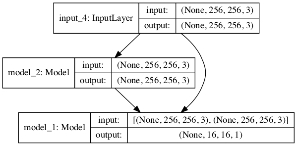
Running the example first summarizes the composite model, showing the 256×256 image input, the same shaped output from model_2 (the generator) and the PatchGAN classification prediction from model_1 (the discriminator).
A plot of the composite model is also created, showing how the input image flows into the generator and discriminator, and that the model has two outputs or end-points from each of the two models.
Note: creating the plot assumes that pydot and pygraphviz libraries are installed. If this is a problem, you can comment out the import and call to the plot_model() function.
Plot of the Composite GAN Model Used to Train the Generator in the Pix2Pix GAN Architecture
How to Update Model Weights
Training the defined models is relatively straightforward.
First, we must define a helper function that will select a batch of real source and target images and the associated output (1.0). Here, the dataset is a list of two arrays of images.
1
2
3
4
5
6
7
8
9
10
11
# select a batch of random samples, returns images and target
Similarly, we need a function to generate a batch of fake images and the associated output (0.0). Here, the samples are an array of source images for which target images will be generated.
1
2
3
4
5
6
7
# generate a batch of images, returns images and targets
Now, we can define the steps of a single training iteration.
First, we must select a batch of source and target images by calling generate_real_samples().
Typically, the batch size (n_batch) is set to 1. In this case, we will assume 256×256 input images, which means the n_patch for the PatchGAN discriminator will be 16 to indicate a 16×16 output feature map.
So far, this is normal for updating a GAN in Keras.
Next, we can update the generator model via adversarial loss and L1 loss. Recall that the composite GAN model takes a batch of source images as input and predicts first the classification of real/fake and second the generated target. Here, we provide a target to indicate the generated images are “real” (class=1) to the discriminator output of the composite model. The real target images are provided for calculating the L1 loss between them and the generated target images.
We have two loss functions, but three loss values calculated for a batch update, where only the first loss value is of interest as it is the weighted sum of the adversarial and L1 loss values for the batch.
We can define all of this in a function called train() that takes the defined models and a loaded dataset (as a list of two NumPy arrays) and trains the models.
I want to ask that you say that unpack dataset. But I cannot figure out how to load the dataset. As far as I understand we should have two datasets, one is the source data that will be translated to the expected images, and the other one is the real images those are used for applying to the source images. But how do we load these datasets?
# load image data
dataset = … (should we type here both of the directories of the datasets?, but I cannot figure out how)
When you set Trainable = False for the discriminator, doesn’t it remain untrainable for all future training batches? Shouldn’t you set Trainable to True every time you’re about to train the discriminator and change it to False every time you train the overall Gan model?
Isn’t the effective receptive field of this discriminator that you wrote 142? because we’ve got 4 convolutional layers with kernel size 4 and stride 2, and two last layers with kernel size 4 and stride 1 which makes the receptive field 142.
Hi Jason,
I have a question regarding the receptive field calculation. I still do not understand why there are 6 conv layers in the implementation code for the 70X70 PatchGAN, but when calculating the receptive field there are only 5 conv layers used. For what purpose one (filter size = 4, stride = 2) conv layer is missed? Can you give me an explanation in detail? Thanks.
Thank you about this article. it is a very useful and i understand from here pix2pix model. IS there any article about Star GAN using keras? https://arxiv.org/abs/1711.09020
thanks once again for an awesome tutorial.
I was wondering if it is possible to save the state of the discriminator, generator and Gan, load them sometime later and continue training ?
thanks for your input. Do you have any code example of saving all three models, loading them and then training again. I tried saving and loading all three models but when attempting to train again the loss of the discriminator and generator was 0 and remained 0. I searched through a lot of forums but to no avail.
Any examples available on this specific topic? I think it would help a great number of people
Hello,
Thank you for the great post!
I have a query about this paragraph:
“We can see that the model output will be an activation map with the size 16×16 pixels or activations and a single channel, with each value in the map corresponding to a 70×70 pixel patch of the input 256×256 image. If the input image was half the size at 128×128, then the output feature map would also be halved to 8×8.”
-> How is it determined that the each value in 16×16 corresponds to a 70×70 pixel patch of input image?
-> what should be the output size if I wanted to apply it for patches of 16×16 of input image?
->does input image mean the one with 256x256x6 (after concatenation) or the one before concatenation?
Hi, In your code, you only take 1 Input layer. How do you take 2 images A and B? I am unable to understand. I’ve been trying to make my own model and this is what I’m doing:
self.discriminator = self.build_discriminator()
self.discriminator.compile(loss=”binary_crossentropy”,
optimizer=optimizer,
loss_weights=[0.5])
print(“## DISCRIMINATOR ##”)
self.discriminator.summary()
# plot_model(self.discriminator, to_file=’discriminator.png’, show_shapes=True, show_layer_names=True)
I’m trying to reproduce pix2pix using pytorch, but when I’m going to implement the discriminator, if I consider the last two layers with kernel size = 4 and stride = 1, the output must be a 14×14 matrix (considering that padding = 1 in the official github project). I can’t understand how padding=’same’ make it keep 16×16.
Hi Jason, I have a question about 70×70 PatchGAN receptive field. In the pix2pix paper, their architecture is C64-C128-C256-C512-C1, all convolution layer have 4×4 filter with stride 2 (page 16), which is a bit different from your implemetation. Following the receptive field calculation, I got:
No, but if you check the code they use a patchgan and don’t include a block before the output layer in their paper description. The implementation I propose is based on the code they released.
Dear author, I face difficult about load and save the GAN in doing my research. So Could you answer me about all type of GAN can save the model and load again.Thank you so much that you give me a chance to leave a Reply to u.
Alright, Thanks for clearing that up, Jason. Also, I noticed there isn’t anything specified for metrics in the compile functions. Are we supposed to leave that blank in GAN/ image generation problems ?
how does the combined Model know on which output to perform which loss? Is it the order of the losses? So the first loss (“binary cross entropy”) will be calculated for the first argument of the output and mae will be calculated for the second?
What do I do then if I want to calculate multiple losses for one of the outputs?
Hi Jason,
Can you implement a Unpaired image to image translation using GAN in tensorflow using resnet block. As I wanted to learn this. Please if you can build a model from scratch it will be helpful.
Thanks for the informative tutorial. I am trying to use this for an image with size 81*81 instead of 256*256, but I am having a few problems. The most important issue is the inconsistent dimension for Conv2DTranspose.
Are there any adjustments that should be done for this specific size?
I am trying to fit a UNet CNN to a task very similar to image to image translation. The input to the network is a binary matrix of size (64,256) and the output is of size (64,32). The accuracy on the training data is around 90% while the accuracy on the test is around 50%. By accuracy here, I mean the average percentage of correct entries in each image. Also, while training the validation loss increases while the loss decreases which is a clear sign of overfitting. I have tried most of the regularization techniques and also tried reducing the capacity of the model but this only reduces the training error while not improving the generalization error. Any advice or ideas?
Thanks a lot for the lesson. I tried to plot the composite (GAN) model without changing anything of your code but I got the following error:
AttributeError: ‘ListWrapper’ object has no attribute ‘name’
Hi Jason. I am trying to add gradient penalty, based on https://jleinonen.github.io/2019/11/07/gan-elements-2.html and Wasserstein loss ( from one of your articles). I am confused about how to modify the discriminator’s train_on_batch. Could you give me a few pointers?
In section : How to Update Model Weights
In the final code:
def train ():
g_loss, _, _ = gan_model.train_on_batch(X_realA, [y_real, X_realB])
.
.
Now in the gan_model():
model = Model(in_src, [dis_out, gen_out])
.
.
Its gen_out == its the output of the gen
BUT in g_loss, _, _ = gan_model.train_on_batch(X_realA, [y_real, X_realB])
Its assigned as:
gen_out = X_realB. this is puzzling me as X_realB is the “target” real img.
.
gen_out is output of the generator.
In the train function
X_fakeB is the “target” img generated by the generator.
Then why is X_realB is used instead of X_fakeB ?
.
Here you’ve mentioned that the ‘patch_shape’ parameter in ‘generate_fake_samples’ and ‘generate_real_samples’ is to be passed as 16 in the section of ‘How to Update Model Weights’, but your other post passes a patch_shape of 1 for those functions. Could you clear out the difference in both examples please? Would be of great help.
As far as I’ve understood, the architecture for the patch GAN discriminator is the same in both the posts. Patch_shape of 16 makes sense as you explain it here, but patch_shape of 1 is a bit confusing.
Perhaps the above example where we work through how the patch gan receptive field is calculated will help? Try working through that part of the tutorial.
You’ve taken the same patch_shape parameter as 1. ( in function summarize_performance(), 1st and 2nd line of code). Is there a difference that I’ve missed somewhere?
Hi Jason.
I reviewed almost all questions in different tutorials but didn’t find my answer.
I want to use images of size 52*52*1 and can’t resize it to 256*256, so I guess I have to change the model itself.
If I try to run it with only the input image size as changes, I’ve got some problem during concatenation: (None, 2, 2, 512) from one side and (None, 1, 1, 512) from the other. I think I have to remove some layers so this is what I tried naively and the same kind of error still remains until I only kept one encoding layer and one decoding layer. Is that the correct way to modify the model according to a smaller size of input images?
What do I have to change as well? the “512” into the bottleneck?
Thank you in advance for your reply as accurate as possible!
I can’t thank you enough for these great tutorials.
There is just a minor typo that i want to correct.
while defining the the first block of decoder in the U-net generator, you said that
“Batch normalization is not used in the first layer of the decoder.”
However, batch normalization is used in the first layer of the decoder. I believe it should be encoder but not the decoder, because batch normalization is not used in the first layer of encoder C64.
Hi Jason!
It was a very helpful tutorial. I learnt and modified the code according to my requirements but when I was training the model, it was very slow. I had 380 training examples and 100 epochs of batch size 1, which was making the number of iterations as big as 38000.
I saw your image translation code and you trained it for approximately 100K iterations. How was your training time? Maybe I did some mistake.
Thanks for the great tutorial. I learned so much from this one
I have implemented your code and added a line to save the whole GAN model ( gan_name = ‘GAN_%06d.h5’ % (step+1) and gan_model.save(gan_name) in summarize_performance ) but when I load the model and continue training the discriminator losses very quickly go down to 0. If I don’t load the model and just train then everything is fine. If we just load the d and g weights then I think the Adam decay resets back to the beta_1 parameter at the beginning.
I saved the GAN model so it remembers the state of the Adam decay, but I’m not sure why this causes the model to stop learning only after loading. I have probably made a mistake but I can’t figure out where.
Could you please extend this tutorial a little bit and show us how to save and resume training for this model in particular please? I’m sure it would be a great help to everyone since Google Colab and many people’s computers can’t be left on for extended periods of time and must be resumed later on
This would really be greatly appreciated from everyone I’m sure
Thanks!
I found that using TensorFlow Checkpoints will enable you to save all the hyperparameter states and allows for restoration of optimisers too, if they are noted in the checkpoint after their instantiation:
Thanks for this tutorial.
I want to use pix2pix for removing watermark from images.
My dataset has 60K samples with 160 different colored watermarks.
I trained pix2pix for about 40000 steps, but nothing happened and the output of the generator is same as input without any changes.
I was wondering if you help me.
I don’t think I will provide detailed help. But pix2pix is a GAN, you should check if your encoder and decoder part are built correctly. Also to verify that the input and output are NOT the same, verify not the visual appearance but the numerical value. You may be just not trained enough.
hi, I am also trying to do oix2pix gan for removing the watermark. I have just started. can you tell me if I should continue with pix2pix gan, or I should change it?
Your detailed explanation is awesome. I used your code structure but I coded it in pytorch in my way. It works like a charm. Your tutorial made me to make awesome results.
Thank you


 From Scratch in Keras")
 From Scratch with Keras")


Does this book cover tensorflow 2.0?
No, tensorflow 2.0 is not released, it is still in beta.
Good????
Thanks!
You are the best.
Thanks!
Let’s say that I want to save the best model. Which loss should I consider to save the model or even to do an early stopping?
Ouch. Excellent question!
Neither. Loss is not a good indicator of GAN generated image quality. WGAN loss can be, LS loss can be, but I would not rely on them in practice.
Instead, save models all the time – like each cycle, use them to generate samples, and select models based on the quality of generated samples.
Evaluate samples with humans or with metrics like incept score or FID (tutorials coming on this).
Thanks for your great contribution.
I want to ask that you say that unpack dataset. But I cannot figure out how to load the dataset. As far as I understand we should have two datasets, one is the source data that will be translated to the expected images, and the other one is the real images those are used for applying to the source images. But how do we load these datasets?
# load image data
dataset = … (should we type here both of the directories of the datasets?, but I cannot figure out how)
sorry if my question is weird.
Correct, the dataset contains paired images.
I give a complete example with a real dataset here:
https://machinelearningmastery.com/how-to-develop-a-pix2pix-gan-for-image-to-image-translation/
When you set Trainable = False for the discriminator, doesn’t it remain untrainable for all future training batches? Shouldn’t you set Trainable to True every time you’re about to train the discriminator and change it to False every time you train the overall Gan model?
Yes, but only in the composite model.
The standalone discriminator is unaffected.
Why batch size of GAN is mostly 1?
Not always, but in this case because we update for each image.
Where do you used lambda?
I am unable to see that one parameter.
Great question, in the loss_weights argument to compile().
Hi Adrian,
Thanks for your great post.
Is there any way to write the code through a negative loss weight for the discriminator rather than interchanging the labels?
Yes, but I don’t have a worked example, sorry.
Sorry , I was going to comment for “How to Code the GAN Training Algorithm and Loss Functions”. It was my fault.
No problem.
Dear Jason,
Isn’t the effective receptive field of this discriminator that you wrote 142? because we’ve got 4 convolutional layers with kernel size 4 and stride 2, and two last layers with kernel size 4 and stride 1 which makes the receptive field 142.
No, the worked example starts at the first conv, not the pixels.
Dear Jason
in ‘Image-to-Image Translation with Conditional Adversarial Networks’ paper:
The 70 * 70 discriminator architecture is:
C64-C128-C256-C512
After the last layer, a convolution is applied to map to
a 1-dimensional output, followed by a Sigmoid function.
but there are two C512 layer in your implementation
i dont understant it …
Thanks for your Great site
Yes, the implementation matches the code they provided where the final C512 “interprets” the 70×70 output.
Hi Jason,
I have a question regarding the receptive field calculation. I still do not understand why there are 6 conv layers in the implementation code for the 70X70 PatchGAN, but when calculating the receptive field there are only 5 conv layers used. For what purpose one (filter size = 4, stride = 2) conv layer is missed? Can you give me an explanation in detail? Thanks.
The final layer interprets the receptive field, matching the paper and official implementation.
This is also noted in the code comments.
Thanks for this excellent resource!
If I print out the model in the author’s original implementation using torch_summary it doesn’t seem to have this additional C512 layer.
—————————————————————-
Layer (type) Output Shape Param #
================================================================
Conv2d-1 [-1, 64, 128, 128] 6,208
LeakyReLU-2 [-1, 64, 128, 128] 0
Conv2d-3 [-1, 128, 64, 64] 131,072
BatchNorm2d-4 [-1, 128, 64, 64] 256
LeakyReLU-5 [-1, 128, 64, 64] 0
Conv2d-6 [-1, 256, 32, 32] 524,288
BatchNorm2d-7 [-1, 256, 32, 32] 512
LeakyReLU-8 [-1, 256, 32, 32] 0
Conv2d-9 [-1, 512, 31, 31] 2,097,152
BatchNorm2d-10 [-1, 512, 31, 31] 1,024
LeakyReLU-11 [-1, 512, 31, 31] 0
Conv2d-12 [-1, 1, 30, 30] 8,193
================================================================
Total params: 2,768,705
Note that it has ~4M fewer parameters too that are added by that extra conv2d layer.
Thank you Jagannath for your feedback!
Dear Jason,
Thank you about this article. it is a very useful and i understand from here pix2pix model. IS there any article about Star GAN using keras?
https://arxiv.org/abs/1711.09020
Thank you
Thanks for the suggestion, I may cover it in the future.
Hello Jason,
thanks once again for an awesome tutorial.
I was wondering if it is possible to save the state of the discriminator, generator and Gan, load them sometime later and continue training ?
Could you point me in the right direction?
Thank you
Yes, you can use save() on each model:
https://machinelearningmastery.com/save-load-keras-deep-learning-models/
Hi Jason,
thanks for your input. Do you have any code example of saving all three models, loading them and then training again. I tried saving and loading all three models but when attempting to train again the loss of the discriminator and generator was 0 and remained 0. I searched through a lot of forums but to no avail.
Any examples available on this specific topic? I think it would help a great number of people
I have an example of training, saving, loading and using the models here:
https://machinelearningmastery.com/how-to-develop-a-pix2pix-gan-for-image-to-image-translation/
In all examples the generator model is only saved and loaded AFTER training to predict / generate new images. Thanks for your tutorials anyway Jason.
Dear Jason,
Many thanks. It was so helpful. And what about pix2pixHD?
Thanks!
I hope to cover it in the future.
Hello,
Thank you for the great post!
I have a query about this paragraph:
“We can see that the model output will be an activation map with the size 16×16 pixels or activations and a single channel, with each value in the map corresponding to a 70×70 pixel patch of the input 256×256 image. If the input image was half the size at 128×128, then the output feature map would also be halved to 8×8.”
-> How is it determined that the each value in 16×16 corresponds to a 70×70 pixel patch of input image?
-> what should be the output size if I wanted to apply it for patches of 16×16 of input image?
->does input image mean the one with 256x256x6 (after concatenation) or the one before concatenation?
Thanks a lot!
Thanks.
See the section titled “How to Implement the PatchGAN Discriminator Model” on how the patch gan is calculated. You can plug-in any numbers you wish.
Hi, In your code, you only take 1 Input layer. How do you take 2 images A and B? I am unable to understand. I’ve been trying to make my own model and this is what I’m doing:
self.discriminator = self.build_discriminator()
self.discriminator.compile(loss=”binary_crossentropy”,
optimizer=optimizer,
loss_weights=[0.5])
print(“## DISCRIMINATOR ##”)
self.discriminator.summary()
# plot_model(self.discriminator, to_file=’discriminator.png’, show_shapes=True, show_layer_names=True)
self.generator = self.build_generator()
print(“## GENERATOR ##”)
self.generator.summary()
# plot_model(self.generator, to_file=”generator.png”, show_shapes=True, show_layer_names=True)
lr = Input(shape=self.img_shape)
hr = Input(shape=self.img_shape)
sr = self.generator(lr)
valid = self.discriminator([sr,hr])
self.discriminator.traininable = False
self.combined = Model(inputs=[lr,hr], outputs=[valid,sr])
self.combined.compile(loss=[‘binary_crossentropy’,’mae’],
loss_weights=[1,100],
optimizer=optimizer)
self.combined.summary()
This is the summary of my GAN:
Model: “model_2”
__________________________________________________________________________________________________
Layer (type) Output Shape Param # Connected to
==================================================================================================
input_4 (InputLayer) [(None, 512, 512, 3) 0
__________________________________________________________________________________________________
model_1 (Model) (None, 512, 512, 3) 54429315 input_4[0][0]
__________________________________________________________________________________________________
input_5 (InputLayer) [(None, 512, 512, 3) 0
__________________________________________________________________________________________________
model (Model) (None, 32, 32, 1) 6968257 model_1[1][0]
input_5[0][0]
==================================================================================================
Total params: 61,397,572
Trainable params: 61,384,900
Non-trainable params: 12,672
I don’t understand how taking 2 Input layers is bad? Why is my discriminator not accepting trainable=False?
Can you please clear my doubts?
I’m eager to help, but I don’t have the capacity to debug your code.
Perhaps the suggestions here will help:
https://machinelearningmastery.com/faq/single-faq/can-you-read-review-or-debug-my-code
Thank you for this wonderful post.
Is it necessary to feed images of 256x256x3 as input ??
Can we feed an image of different sizes like 480x480x3 ??
Instead of a square image can we feed a non-square image to the network??
Yes, but you will need to change the model.
Please explain what and wherein model-network changes will be required for and square or non-square images.
Sorry, I don’t have the capacity to customize the example for you.
REALLY useful information!
I’ve made one small change for my b/w dataset, based on the line:
“After the last layer in the decoder, a convolution is applied to map to the number of output channels (3 in general […])”
I’m training some b/w data, shape [256,256,1] and notice that there is one hard-coded “3”
in define_generator at the end:
g = Conv2DTranspose(3, (4,4), strides=(2,2), padding=’same’, kernel_initializer=init)(d7)
You default to 3-channel images, but your input_shape can handle other variations with this modest change:
g = Conv2DTranspose(input_shape[2], (4,4), strides=(2,2), padding=’same’, kernel_initializer=init)(d7)
Thanks for making this
Thanks!
Great suggestion Scott.
Hello, I would like to ask a question.
I’m trying to reproduce pix2pix using pytorch, but when I’m going to implement the discriminator, if I consider the last two layers with kernel size = 4 and stride = 1, the output must be a 14×14 matrix (considering that padding = 1 in the official github project). I can’t understand how padding=’same’ make it keep 16×16.
Perhaps use an existing pytorch implementation of the model?
What is the purpose of concatenating the real and generated images when passed as input to the discriminator?
To have both images types in the batch when updating weights.
Hi Jason, I have a question about 70×70 PatchGAN receptive field. In the pix2pix paper, their architecture is C64-C128-C256-C512-C1, all convolution layer have 4×4 filter with stride 2 (page 16), which is a bit different from your implemetation. Following the receptive field calculation, I got:
receptive_field(1, 4, 2)
Out[3]: 4
receptive_field(4, 4, 2)
Out[4]: 10
receptive_field(10, 4, 2)
Out[5]: 22
receptive_field(22, 4, 2)
Out[6]: 46
receptive_field(46, 4, 2)
Out[7]: 94
Did they change the architecture?
No, but if you check the code they use a patchgan and don’t include a block before the output layer in their paper description. The implementation I propose is based on the code they released.
Dear author, I face difficult about load and save the GAN in doing my research. So Could you answer me about all type of GAN can save the model and load again.Thank you so much that you give me a chance to leave a Reply to u.
You can see examples here:
https://machinelearningmastery.com/how-to-develop-a-pix2pix-gan-for-image-to-image-translation/
Can you share a link from where I can download this model (Github or Some online storage link).
No. I do not share the trained model. My focus is on helping developers build the models and models like it.
why your site ban Iran country ip?
we are just eager students and your site is very helpful.
Some governments have blocked access to my site, no idea why:
https://machinelearningmastery.com/faq/single-faq/why-is-your-website-blocked-in-my-country
How do we work with images that are larger than 256×256 and not necessarily square?
Either scale the images to match the model or change the model to match the images.
Hi Jason. Shouldn’t one use a custom loss function instead of mae in the section, How to Implement Adversarial and L1 Loss ?
def L1(y_true, y_pred):
x = K.abs(y_true – y_pred)
return K.sum(x)
Something like this instead of mae.
Yes, we do this, see the “mae’ loss used in the composite model.
We use L1 adversarial loss in this case, as is described in the paper.
Alright, Thanks for clearing that up, Jason. Also, I noticed there isn’t anything specified for metrics in the compile functions. Are we supposed to leave that blank in GAN/ image generation problems ?
Yes. Evaluating GANs is really really hard, doing it visually is the most reliable way:
https://machinelearningmastery.com/how-to-evaluate-generative-adversarial-networks/
Hi Jason,
how does the combined Model know on which output to perform which loss? Is it the order of the losses? So the first loss (“binary cross entropy”) will be calculated for the first argument of the output and mae will be calculated for the second?
What do I do then if I want to calculate multiple losses for one of the outputs?
We carefully constructed the model.
Perhaps start with this simpler GAN to understand how the models are related:
https://machinelearningmastery.com/how-to-develop-a-generative-adversarial-network-for-a-1-dimensional-function-from-scratch-in-keras/
Hi Jason,
Can you implement a Unpaired image to image translation using GAN in tensorflow using resnet block. As I wanted to learn this. Please if you can build a model from scratch it will be helpful.
original paper: https://arxiv.org/abs/1703.10593
You can use a cyclegan for unpaired image to image translation:
https://machinelearningmastery.com/cyclegan-tutorial-with-keras/
Hi Jason,
Thanks for the informative tutorial. I am trying to use this for an image with size 81*81 instead of 256*256, but I am having a few problems. The most important issue is the inconsistent dimension for Conv2DTranspose.
Are there any adjustments that should be done for this specific size?
Thank you
You will have to tune the model to the new size. It may require some trial and error.
Hello Jason,
I am trying to fit a UNet CNN to a task very similar to image to image translation. The input to the network is a binary matrix of size (64,256) and the output is of size (64,32). The accuracy on the training data is around 90% while the accuracy on the test is around 50%. By accuracy here, I mean the average percentage of correct entries in each image. Also, while training the validation loss increases while the loss decreases which is a clear sign of overfitting. I have tried most of the regularization techniques and also tried reducing the capacity of the model but this only reduces the training error while not improving the generalization error. Any advice or ideas?
Intersting.
Maybe some of the ideas here could be tried:
https://machinelearningmastery.com/introduction-to-regularization-to-reduce-overfitting-and-improve-generalization-error/
Thanks a lot for the lesson. I tried to plot the composite (GAN) model without changing anything of your code but I got the following error:
AttributeError: ‘ListWrapper’ object has no attribute ‘name’
Sorry to hear that, this might help:
https://machinelearningmastery.com/faq/single-faq/why-does-the-code-in-the-tutorial-not-work-for-me
Hi Jason. I am trying to add gradient penalty, based on https://jleinonen.github.io/2019/11/07/gan-elements-2.html and Wasserstein loss ( from one of your articles). I am confused about how to modify the discriminator’s train_on_batch. Could you give me a few pointers?
Sorry, I am not familiar with that article, perhaps ask the authors directly?
.
Very imp doubt.
In section : How to Update Model Weights
In the final code:
def train ():
g_loss, _, _ = gan_model.train_on_batch(X_realA, [y_real, X_realB])
.
.
Now in the gan_model():
model = Model(in_src, [dis_out, gen_out])
.
.
Its gen_out == its the output of the gen
BUT in g_loss, _, _ = gan_model.train_on_batch(X_realA, [y_real, X_realB])
Its assigned as:
gen_out = X_realB. this is puzzling me as X_realB is the “target” real img.
.
gen_out is output of the generator.
In the train function
X_fakeB is the “target” img generated by the generator.
Then why is X_realB is used instead of X_fakeB ?
.
What is the problem you’re having exactly? Perhaps you can elaborate?
Hi!
Thanks for this wonderful post!
I have a small confusion following this article and this next one:
https://machinelearningmastery.com/how-to-develop-a-pix2pix-gan-for-image-to-image-translation/
Here you’ve mentioned that the ‘patch_shape’ parameter in ‘generate_fake_samples’ and ‘generate_real_samples’ is to be passed as 16 in the section of ‘How to Update Model Weights’, but your other post passes a patch_shape of 1 for those functions. Could you clear out the difference in both examples please? Would be of great help.
As far as I’ve understood, the architecture for the patch GAN discriminator is the same in both the posts. Patch_shape of 16 makes sense as you explain it here, but patch_shape of 1 is a bit confusing.
You’re welcome.
Perhaps the above example where we work through how the patch gan receptive field is calculated will help? Try working through that part of the tutorial.
Yes, I did follow through that example calculation, but here I’m confused about what value does the ‘patch_shape’ parameter takes, in ‘generate_fake_samples’ and ‘generate_real_samples’ ? The output shape of 16×16 makes sense here in this article, but on your previous one here: https://machinelearningmastery.com/how-to-develop-a-pix2pix-gan-for-image-to-image-translation/
You’ve taken the same patch_shape parameter as 1. ( in function summarize_performance(), 1st and 2nd line of code). Is there a difference that I’ve missed somewhere?
No, they are the same I believe.
Hi Jason.
I reviewed almost all questions in different tutorials but didn’t find my answer.
I want to use images of size 52*52*1 and can’t resize it to 256*256, so I guess I have to change the model itself.
If I try to run it with only the input image size as changes, I’ve got some problem during concatenation: (None, 2, 2, 512) from one side and (None, 1, 1, 512) from the other. I think I have to remove some layers so this is what I tried naively and the same kind of error still remains until I only kept one encoding layer and one decoding layer. Is that the correct way to modify the model according to a smaller size of input images?
What do I have to change as well? the “512” into the bottleneck?
Thank you in advance for your reply as accurate as possible!
Yes, you many (will!) need to customise the number and size of layers to achieve your desired inputs and outputs.
I can’t thank you enough for these great tutorials.
There is just a minor typo that i want to correct.
while defining the the first block of decoder in the U-net generator, you said that
“Batch normalization is not used in the first layer of the decoder.”
However, batch normalization is used in the first layer of the decoder. I believe it should be encoder but not the decoder, because batch normalization is not used in the first layer of encoder C64.
Thank you!
Thanks, fixed!
Hi Jason!
It was a very helpful tutorial. I learnt and modified the code according to my requirements but when I was training the model, it was very slow. I had 380 training examples and 100 epochs of batch size 1, which was making the number of iterations as big as 38000.
I saw your image translation code and you trained it for approximately 100K iterations. How was your training time? Maybe I did some mistake.
I don’t recall sorry, I think I trained overnight on an AWS EC2 instance.
My g_loss is way too high around 17000. Earlier I was running the model on CPU, but now I switched to GPU and it’s much faster now.
Loss may not be a good sign of GAN model performance. Look at the generated images.
Hi Jason,
Thanks for the great tutorial. I learned so much from this one
I have implemented your code and added a line to save the whole GAN model ( gan_name = ‘GAN_%06d.h5’ % (step+1) and gan_model.save(gan_name) in summarize_performance ) but when I load the model and continue training the discriminator losses very quickly go down to 0. If I don’t load the model and just train then everything is fine. If we just load the d and g weights then I think the Adam decay resets back to the beta_1 parameter at the beginning.
I saved the GAN model so it remembers the state of the Adam decay, but I’m not sure why this causes the model to stop learning only after loading. I have probably made a mistake but I can’t figure out where.
Could you please extend this tutorial a little bit and show us how to save and resume training for this model in particular please? I’m sure it would be a great help to everyone since Google Colab and many people’s computers can’t be left on for extended periods of time and must be resumed later on
This would really be greatly appreciated from everyone I’m sure
Thanks!
Thanks for your suggestion. This is something we planned to write.
Hi Adrian,
I found that using TensorFlow Checkpoints will enable you to save all the hyperparameter states and allows for restoration of optimisers too, if they are noted in the checkpoint after their instantiation:
checkpoint = tf.train.Checkpoint(generator_optimizer=generator_optimizer, discriminator_optimizer=discriminator_optimizer, generator=generator, discriminator=discriminator)
and then:
checkpoint.save(…)
Hi Jason,
Thanks for this tutorial.
I want to use pix2pix for removing watermark from images.
My dataset has 60K samples with 160 different colored watermarks.
I trained pix2pix for about 40000 steps, but nothing happened and the output of the generator is same as input without any changes.
I was wondering if you help me.
I don’t think I will provide detailed help. But pix2pix is a GAN, you should check if your encoder and decoder part are built correctly. Also to verify that the input and output are NOT the same, verify not the visual appearance but the numerical value. You may be just not trained enough.
hi, I am also trying to do oix2pix gan for removing the watermark. I have just started. can you tell me if I should continue with pix2pix gan, or I should change it?
Hi Adrian,
Your detailed explanation is awesome. I used your code structure but I coded it in pytorch in my way. It works like a charm. Your tutorial made me to make awesome results.
Thank you
Not Adrian, sorry for Typo. The credit goes to Jason Brownlee
Your explanation is so easy and helpful to understand.
I would like to run the above code.
Could you tell me if the above code works?
Thank you.
Hi YooJC…Thank you for your feedback! Please feel free to execute the code and let us know your findings.