It is an effective approach for time series forecasting, although it requires careful analysis and domain expertise in order to configure the seven or more model hyperparameters.
An alternative approach to configuring the model that makes use of fast and parallel modern hardware is to grid search a suite of hyperparameter configurations in order to discover what works best. Often, this process can reveal non-intuitive model configurations that result in lower forecast error than those configurations specified through careful analysis.
In this tutorial, you will discover how to develop a framework for grid searching all of the SARIMA model hyperparameters for univariate time series forecasting.
After completing this tutorial, you will know:
How to develop a framework for grid searching SARIMA models from scratch using walk-forward validation.
How to grid search SARIMA model hyperparameters for daily time series data for births.
How to grid search SARIMA model hyperparameters for monthly time series data for shampoo sales, car sales, and temperature.
Kick-start your project with my new book Deep Learning for Time Series Forecasting, including step-by-step tutorials and the Python source code files for all examples.
Let’s get started.
Updated Apr/2019: Updated the link to dataset.
How to Grid Search SARIMA Model Hyperparameters for Time Series Forecasting in Python Photo by Thomas, some rights reserved.
Tutorial Overview
This tutorial is divided into six parts; they are:
SARIMA for Time Series Forecasting
Develop a Grid Search Framework
Case Study 1: No Trend or Seasonality
Case Study 2: Trend
Case Study 3: Seasonality
Case Study 4: Trend and Seasonality
SARIMA for Time Series Forecasting
Seasonal Autoregressive Integrated Moving Average, SARIMA or Seasonal ARIMA, is an extension of ARIMA that explicitly supports univariate time series data with a seasonal component.
It adds three new hyperparameters to specify the autoregression (AR), differencing (I), and moving average (MA) for the seasonal component of the series, as well as an additional parameter for the period of the seasonality.
A seasonal ARIMA model is formed by including additional seasonal terms in the ARIMA […] The seasonal part of the model consists of terms that are very similar to the non-seasonal components of the model, but they involve backshifts of the seasonal period.
Configuring a SARIMA requires selecting hyperparameters for both the trend and seasonal elements of the series.
There are three trend elements that require configuration.
They are the same as the ARIMA model; specifically:
p: Trend autoregression order.
d: Trend difference order.
q: Trend moving average order.
There are four seasonal elements that are not part of ARIMA that must be configured; they are:
P: Seasonal autoregressive order.
D: Seasonal difference order.
Q: Seasonal moving average order.
m: The number of time steps for a single seasonal period.
Together, the notation for a SARIMA model is specified as:
1
SARIMA(p,d,q)(P,D,Q)m
The SARIMA model can subsume the ARIMA, ARMA, AR, and MA models via model configuration parameters.
The trend and seasonal hyperparameters of the model can be configured by analyzing autocorrelation and partial autocorrelation plots, and this can take some expertise.
An alternative approach is to grid search a suite of model configurations and discover which configurations work best for a specific univariate time series.
Seasonal ARIMA models can potentially have a large number of parameters and combinations of terms. Therefore, it is appropriate to try out a wide range of models when fitting to data and choose a best fitting model using an appropriate criterion …
This approach can be faster on modern computers than an analysis process and can reveal surprising findings that might not be obvious and result in lower forecast error.
Need help with Deep Learning for Time Series?
Take my free 7-day email crash course now (with sample code).
Click to sign-up and also get a free PDF Ebook version of the course.
Develop a Grid Search Framework
In this section, we will develop a framework for grid searching SARIMA model hyperparameters for a given univariate time series forecasting problem.
We will use the implementation of SARIMA provided by the statsmodels library.
This model has hyperparameters that control the nature of the model performed for the series, trend and seasonality, specifically:
order: A tuple p, d, and q parameters for the modeling of the trend.
sesonal_order: A tuple of P, D, Q, and m parameters for the modeling the seasonality
trend: A parameter for controlling a model of the deterministic trend as one of ‘n’,’c’,’t’,’ct’ for no trend, constant, linear, and constant with linear trend, respectively.
If you know enough about your problem to specify one or more of these parameters, then you should specify them. If not, you can try grid searching these parameters.
We can start-off by defining a function that will fit a model with a given configuration and make a one-step forecast.
The sarima_forecast() below implements this behavior.
The function takes an array or list of contiguous prior observations and a list of configuration parameters used to configure the model, specifically two tuples and a string for the trend order, seasonal order trend, and parameter.
We also try to make the model robust by relaxing constraints, such as that the data must be stationary and that the MA transform be invertible.
Next, we need to build up some functions for fitting and evaluating a model repeatedly via walk-forward validation, including splitting a dataset into train and test sets and evaluating one-step forecasts.
We can split a list or NumPy array of data using a slice given a specified size of the split, e.g. the number of time steps to use from the data in the test set.
The train_test_split() function below implements this for a provided dataset and a specified number of time steps to use in the test set.
1
2
3
# split a univariate dataset into train/test sets
def train_test_split(data,n_test):
returndata[:-n_test],data[-n_test:]
After forecasts have been made for each step in the test dataset, they need to be compared to the test set in order to calculate an error score.
There are many popular error scores for time series forecasting. In this case we will use root mean squared error (RMSE), but you can change this to your preferred measure, e.g. MAPE, MAE, etc.
The measure_rmse() function below will calculate the RMSE given a list of actual (the test set) and predicted values.
1
2
3
# root mean squared error or rmse
def measure_rmse(actual,predicted):
returnsqrt(mean_squared_error(actual,predicted))
We can now implement the walk-forward validation scheme. This is a standard approach to evaluating a time series forecasting model that respects the temporal ordering of observations.
First, a provided univariate time series dataset is split into train and test sets using the train_test_split() function. Then the number of observations in the test set are enumerated. For each we fit a model on all of the history and make a one step forecast. The true observation for the time step is then added to the history and the process is repeated. The sarima_forecast() function is called in order to fit a model and make a prediction. Finally, an error score is calculated by comparing all one-step forecasts to the actual test set by calling the measure_rmse() function.
The walk_forward_validation() function below implements this, taking a univariate time series, a number of time steps to use in the test set, and an array of model configuration.
1
2
3
4
5
6
7
8
9
10
11
12
13
14
15
16
17
18
# walk-forward validation for univariate data
def walk_forward_validation(data,n_test,cfg):
predictions=list()
# split dataset
train,test=train_test_split(data,n_test)
# seed history with training dataset
history=[xforxintrain]
# step over each time-step in the test set
foriinrange(len(test)):
# fit model and make forecast for history
yhat=sarima_forecast(history,cfg)
# store forecast in list of predictions
predictions.append(yhat)
# add actual observation to history for the next loop
history.append(test[i])
# estimate prediction error
error=measure_rmse(test,predictions)
returnerror
If you are interested in making multi-step predictions, you can change the call to predict() in the sarima_forecast() function and also change the calculation of error in the measure_rmse() function.
We can call walk_forward_validation() repeatedly with different lists of model configurations.
One possible issue is that some combinations of model configurations may not be called for the model and will throw an exception, e.g. specifying some but not all aspects of the seasonal structure in the data.
Further, some models may also raise warnings on some data, e.g. from the linear algebra libraries called by the statsmodels library.
We can trap exceptions and ignore warnings during the grid search by wrapping all calls to walk_forward_validation() with a try-except and a block to ignore warnings. We can also add debugging support to disable these protections in the case we want to see what is really going on. Finally, if an error does occur, we can return a None result, otherwise we can print some information about the skill of each model evaluated. This is helpful when a large number of models are evaluated.
The score_model() function below implements this and returns a tuple of (key and result), where the key is a string version of the tested model configuration.
1
2
3
4
5
6
7
8
9
10
11
12
13
14
15
16
17
18
19
20
21
# score a model, return None on failure
def score_model(data,n_test,cfg,debug=False):
result=None
# convert config to a key
key=str(cfg)
# show all warnings and fail on exception if debugging
ifdebug:
result=walk_forward_validation(data,n_test,cfg)
else:
# one failure during model validation suggests an unstable config
try:
# never show warnings when grid searching, too noisy
with catch_warnings():
filterwarnings("ignore")
result=walk_forward_validation(data,n_test,cfg)
except:
error=None
# check for an interesting result
ifresult isnotNone:
print(' > Model[%s] %.3f'%(key,result))
return(key,result)
Next, we need a loop to test a list of different model configurations.
This is the main function that drives the grid search process and will call the score_model() function for each model configuration.
We can dramatically speed up the grid search process by evaluating model configurations in parallel. One way to do that is to use the Joblib library.
We can define a Parallel object with the number of cores to use and set it to the number of scores detected in your hardware.
We can then can then create a list of tasks to execute in parallel, which will be one call to the score_model() function for each model configuration we have.
The result of evaluating a list of configurations will be a list of tuples, each with a name that summarizes a specific model configuration and the error of the model evaluated with that configuration as either the RMSE or None if there was an error.
We can filter out all scores with a None.
1
scores=[rforrinscores ifr[1]!=None]
We can then sort all tuples in the list by the score in ascending order (best are first), then return this list of scores for review.
The grid_search() function below implements this behavior given a univariate time series dataset, a list of model configurations (list of lists), and the number of time steps to use in the test set. An optional parallel argument allows the evaluation of models across all cores to be tuned on or off, and is on by default.
The only thing left to do is to define a list of model configurations to try for a dataset.
We can define this generically. The only parameter we may want to specify is the periodicity of the seasonal component in the series, if one exists. By default, we will assume no seasonal component.
The sarima_configs() function below will create a list of model configurations to evaluate.
The configurations assume each of the AR, MA, and I components for trend and seasonality are low order, e.g. off (0) or in [1,2]. You may want to extend these ranges if you believe the order may be higher. An optional list of seasonal periods can be specified, and you could even change the function to specify other elements that you may know about your time series.
In theory, there are 1,296 possible model configurations to evaluate, but in practice, many will not be valid and will result in an error that we will trap and ignore.
1
2
3
4
5
6
7
8
9
10
11
12
13
14
15
16
17
18
19
20
21
22
23
24
# create a set of sarima configs to try
def sarima_configs(seasonal=[0]):
models=list()
# define config lists
p_params=[0,1,2]
d_params=[0,1]
q_params=[0,1,2]
t_params=['n','c','t','ct']
P_params=[0,1,2]
D_params=[0,1]
Q_params=[0,1,2]
m_params=seasonal
# create config instances
forpinp_params:
fordind_params:
forqinq_params:
fortint_params:
forPinP_params:
forDinD_params:
forQinQ_params:
forminm_params:
cfg=[(p,d,q),(P,D,Q,m),t]
models.append(cfg)
returnmodels
We now have a framework for grid searching SARIMA model hyperparameters via one-step walk-forward validation.
It is generic and will work for any in-memory univariate time series provided as a list or NumPy array.
We can make sure all the pieces work together by testing it on a contrived 10-step dataset.
The complete example is listed below.
1
2
3
4
5
6
7
8
9
10
11
12
13
14
15
16
17
18
19
20
21
22
23
24
25
26
27
28
29
30
31
32
33
34
35
36
37
38
39
40
41
42
43
44
45
46
47
48
49
50
51
52
53
54
55
56
57
58
59
60
61
62
63
64
65
66
67
68
69
70
71
72
73
74
75
76
77
78
79
80
81
82
83
84
85
86
87
88
89
90
91
92
93
94
95
96
97
98
99
100
101
102
103
104
105
106
107
108
109
110
111
112
113
114
115
116
117
118
119
120
121
122
123
124
125
# grid search sarima hyperparameters
from math import sqrt
from multiprocessing import cpu_count
from joblib import Parallel
from joblib import delayed
from warnings import catch_warnings
from warnings import filterwarnings
from statsmodels.tsa.statespace.sarimax import SARIMAX
Running the example first prints the contrived time series dataset.
Next, the model configurations and their errors are reported as they are evaluated, truncated below for brevity.
Finally, the configurations and the error for the top three configurations are reported. We can see that many models achieve perfect performance on this simple linearly increasing contrived time series problem.
Now that we have a robust framework for grid searching SARIMA model hyperparameters, let’s test it out on a suite of standard univariate time series datasets.
The datasets were chosen for demonstration purposes; I am not suggesting that a SARIMA model is the best approach for each dataset; perhaps an ETS or something else would be more appropriate in some cases.
Case Study 1: No Trend or Seasonality
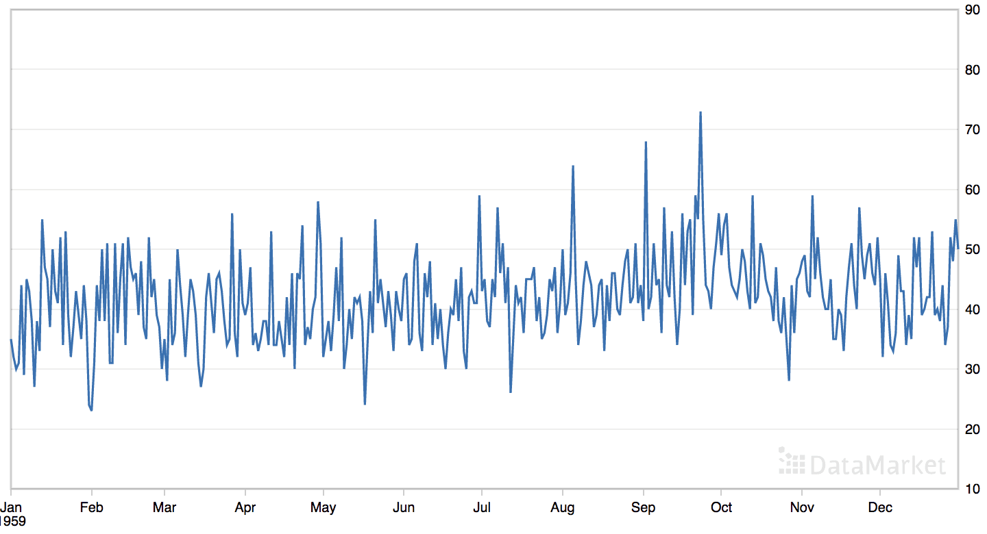
The ‘daily female births’ dataset summarizes the daily total female births in California, USA in 1959.
The dataset has no obvious trend or seasonal component.
Running the example may take a few minutes on modern hardware.
Model configurations and the RMSE are printed as the models are evaluated The top three model configurations and their error are reported at the end of the run.
Note: Your results may vary given the stochastic nature of the algorithm or evaluation procedure, or differences in numerical precision. Consider running the example a few times and compare the average outcome.
We can see that the best result was an RMSE of about 6.77 births with the following configuration:
Order: (1, 0, 2)
Seasonal Order: (1, 0, 1, 0)
Trend Parameter: ‘t’ for linear trend
It is surprising that a configuration with some seasonal elements resulted in the lowest error. I would not have guessed at this configuration and would have likely stuck with an ARIMA model.
1
2
3
4
5
6
7
8
9
10
11
...
> Model[[(2, 1, 2), (1, 0, 1, 0), 'ct']] 6.905
> Model[[(2, 1, 2), (2, 0, 0, 0), 'ct']] 7.031
> Model[[(2, 1, 2), (2, 0, 1, 0), 'ct']] 6.985
> Model[[(2, 1, 2), (1, 0, 2, 0), 'ct']] 6.941
> Model[[(2, 1, 2), (2, 0, 2, 0), 'ct']] 7.056
done
[(1, 0, 2), (1, 0, 1, 0), 't'] 6.770349800255089
[(0, 1, 2), (1, 0, 2, 0), 'ct'] 6.773217122759515
[(2, 1, 1), (2, 0, 2, 0), 'ct'] 6.886633191752254
Case Study 2: Trend
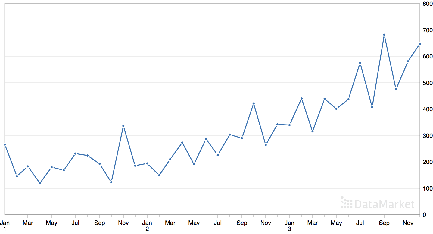
The ‘shampoo’ dataset summarizes the monthly sales of shampoo over a three-year period.
The dataset contains an obvious trend but no obvious seasonal component.
Running the example may take a few minutes on modern hardware.
Model configurations and the RMSE are printed as the models are evaluated The top three model configurations and their error are reported at the end of the run.
Note: Your results may vary given the stochastic nature of the algorithm or evaluation procedure, or differences in numerical precision. Consider running the example a few times and compare the average outcome.
We can see that the best result was an RMSE of about 54.76 sales with the following configuration:
Trend Order: (0, 1, 2)
Seasonal Order: (2, 0, 2, 0)
Trend Parameter: ‘t’ (linear trend)
1
2
3
4
5
6
7
8
9
10
...
> Model[[(2, 1, 2), (1, 0, 1, 0), 'ct']] 68.891
> Model[[(2, 1, 2), (2, 0, 0, 0), 'ct']] 75.406
> Model[[(2, 1, 2), (1, 0, 2, 0), 'ct']] 80.908
> Model[[(2, 1, 2), (2, 0, 1, 0), 'ct']] 78.734
> Model[[(2, 1, 2), (2, 0, 2, 0), 'ct']] 82.958
done
[(0, 1, 2), (2, 0, 2, 0), 't'] 54.767582003072874
[(0, 1, 1), (2, 0, 2, 0), 'ct'] 58.69987083057107
[(1, 1, 2), (0, 0, 1, 0), 't'] 58.709089340600094
Case Study 3: Seasonality
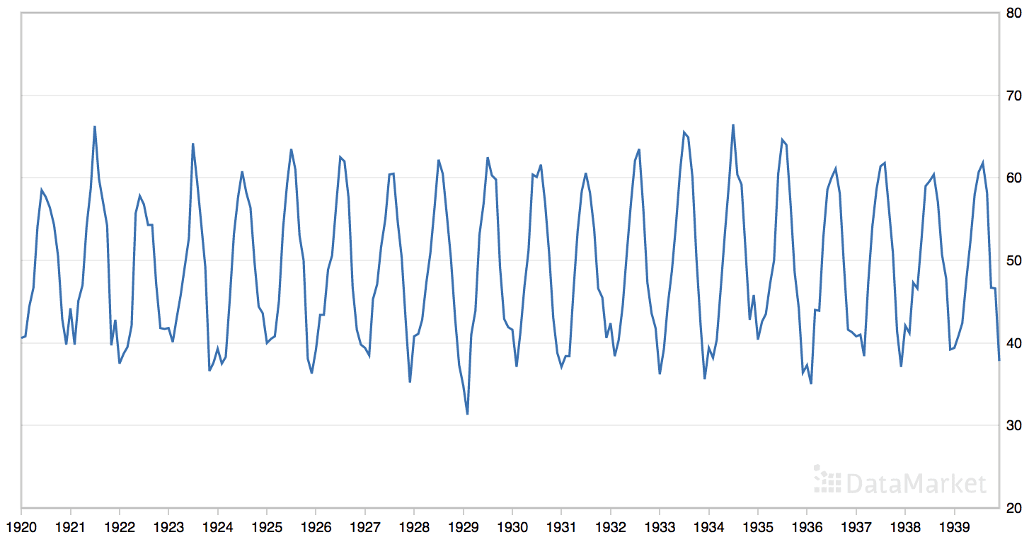
The ‘monthly mean temperatures’ dataset summarizes the monthly average air temperatures in Nottingham Castle, England from 1920 to 1939 in degrees Fahrenheit.
The dataset has an obvious seasonal component and no obvious trend.
Line Plot of the Monthly Mean Temperatures Dataset
The dataset has 20 years, or 240 observations. We will trim the dataset to the last five years of data (60 observations) in order to speed up the model evaluation process and use the last year, or 12 observations, for the test set.
1
2
# trim dataset to 5 years
data=data[-(5*12):]
The period of the seasonal component is about one year, or 12 observations. We will use this as the seasonal period in the call to the sarima_configs() function when preparing the model configurations.
1
2
# model configs
cfg_list=sarima_configs(seasonal=[0,12])
The complete example grid searching the monthly mean temperature time series forecasting problem is listed below.
1
2
3
4
5
6
7
8
9
10
11
12
13
14
15
16
17
18
19
20
21
22
23
24
25
26
27
28
29
30
31
32
33
34
35
36
37
38
39
40
41
42
43
44
45
46
47
48
49
50
51
52
53
54
55
56
57
58
59
60
61
62
63
64
65
66
67
68
69
70
71
72
73
74
75
76
77
78
79
80
81
82
83
84
85
86
87
88
89
90
91
92
93
94
95
96
97
98
99
100
101
102
103
104
105
106
107
108
109
110
111
112
113
114
115
116
117
118
119
120
121
122
123
124
125
126
127
128
# grid search sarima hyperparameters for monthly mean temp dataset
from math import sqrt
from multiprocessing import cpu_count
from joblib import Parallel
from joblib import delayed
from warnings import catch_warnings
from warnings import filterwarnings
from statsmodels.tsa.statespace.sarimax import SARIMAX
Running the example may take a few minutes on modern hardware.
Model configurations and the RMSE are printed as the models are evaluated The top three model configurations and their error are reported at the end of the run.
Note: Your results may vary given the stochastic nature of the algorithm or evaluation procedure, or differences in numerical precision. Consider running the example a few times and compare the average outcome.
We can see that the best result was an RMSE of about 1.5 degrees with the following configuration:
Trend Order: (0, 0, 0)
Seasonal Order: (1, 0, 1, 12)
Trend Parameter: ‘n’ (no trend)
As we would expect, the model has no trend component and a 12-month seasonal ARMA component.
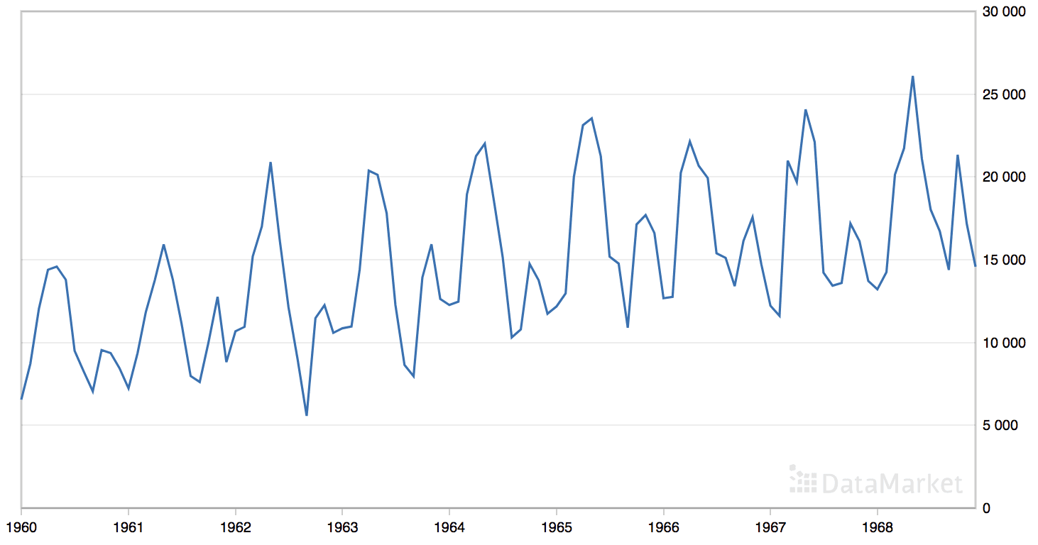
The dataset has 9 years, or 108 observations. We will use the last year, or 12 observations, as the test set.
The period of the seasonal component could be six months or 12 months. We will try both as the seasonal period in the call to the sarima_configs() function when preparing the model configurations.
1
2
# model configs
cfg_list=sarima_configs(seasonal=[0,6,12])
The complete example grid searching the monthly car sales time series forecasting problem is listed below.
1
2
3
4
5
6
7
8
9
10
11
12
13
14
15
16
17
18
19
20
21
22
23
24
25
26
27
28
29
30
31
32
33
34
35
36
37
38
39
40
41
42
43
44
45
46
47
48
49
50
51
52
53
54
55
56
57
58
59
60
61
62
63
64
65
66
67
68
69
70
71
72
73
74
75
76
77
78
79
80
81
82
83
84
85
86
87
88
89
90
91
92
93
94
95
96
97
98
99
100
101
102
103
104
105
106
107
108
109
110
111
112
113
114
115
116
117
118
119
120
121
122
123
124
125
126
127
# grid search sarima hyperparameters for monthly car sales dataset
from math import sqrt
from multiprocessing import cpu_count
from joblib import Parallel
from joblib import delayed
from warnings import catch_warnings
from warnings import filterwarnings
from statsmodels.tsa.statespace.sarimax import SARIMAX
Running the example may take a few minutes on modern hardware.
Model configurations and the RMSE are printed as the models are evaluated The top three model configurations and their error are reported at the end of the run.
Note: Your results may vary given the stochastic nature of the algorithm or evaluation procedure, or differences in numerical precision. Consider running the example a few times and compare the average outcome.
We can see that the best result was an RMSE of about 1,551 sales with the following configuration:
This section lists some ideas for extending the tutorial that you may wish to explore.
Data Transforms. Update the framework to support configurable data transforms such as normalization and standardization.
Plot Forecast. Update the framework to re-fit a model with the best configuration and forecast the entire test dataset, then plot the forecast compared to the actual observations in the test set.
Tune Amount of History. Update the framework to tune the amount of historical data used to fit the model (e.g. in the case of the 10 years of max temperature data).
If you explore any of these extensions, I’d love to know.
Further Reading
This section provides more resources on the topic if you are looking to go deeper.
In this tutorial, you discovered how to develop a framework for grid searching all of the SARIMA model hyperparameters for univariate time series forecasting.
Specifically, you learned:
How to develop a framework for grid searching SARIMA models from scratch using walk-forward validation.
How to grid search SARIMA model hyperparameters for daily time series data for births.
How to grid search SARIMA model hyperparameters for monthly time series data for shampoo sales, car sales and temperature.
Do you have any questions?
Ask your questions in the comments below and I will do my best to answer.
Develop Deep Learning models for Time Series Today!
Many thanks for the article. It’s really impressive, but eight nested for loops are not pythonic. Probably, there is a smarter way to do it. For instance, use ‘itertools.product’
Thanks for this, I’ve been learning about ARIMA for my applications. I learnt a lot from Forecasting Principles and Practice which has an opentexts online version: https://otexts.org/fpp2/arima.html
One of the main issues I have with SARIMA (or maybe it’s just statsmodels) is that it doesn’t handle very large datasets very well. I have timeseries data with records every 5 minutes for ~6 years with 1 day or 1 week season length, ie. monday 9am is likely to correlate with monday 9am next week, which shows up in the differencing and ACF plots. Is there a better way or a better library to do this?
My thoughts: In Model[[(2, 1, 2), (1, 0, 2, 0), ‘ct’]], s=0 (seasonal periodicity) implies that no seasonality. In seasonal config (P,D,Q,s), when s=0, P,D,Q are not interpretable and should be forced to 0. Model[[(2, 1, 2), (1, 0, 2, 0), ‘ct’]] are not meaningful config and should be excluded. Final configu for case 1, especially, ‘ct’, are not intuitive.
Thanks for writing all the procedures step-by-step. However, I tried to run some of the example codes (first one and the last one). I am using Jupyter notebook in Windows 10 and Python 3. Unfortunately, in both cases the notebook was frozen during execution and stayed there forever. Is there something I am missing here?
amazing website about machine learning and your books are fantastic. I am beginner and I am reading all your books and I am trying run programs. I tried run program”Case Study 1: No Trend or Seasonality” on python 3 but program not finishYour program is still running!
Do you want to kill it?) Could you help me? Thx
Thank you so much for the helpful article! I have a question on Case Study 4 – the best fitted model with minimum RMSE has trend order (p=0,d=0,q=0), with d = 0 meaning the model does not need to do first-order differencing to remove trend. However we do observe clear trend in the data. Would this be a conflict? Thanks!
Dear Jason, I have been tryng to export the tuple into a dataframe, but I am unable to do so. In lines 132 and 133 of the case study 2, I changed the code with
for cfg, error in scores[:3]:
df=pd.DataFrame(cfg, error)
output_table = df
I did not wok, so I tried with
for cfg, error in scores[:3]:
df.append({‘cfg’: cfg, ‘error’: error},ignore_index=True)
output_table = df
I know that this is not a Sarima question, but I will appreciate your help
Jason, My question is around the time taken by SARIMA. Is there a way to reduce the search space or the parameter combinations that we are trying? Let me know. Thank you.
Hello Jason, using the grid search code on my dataset only displaying the contrived time series data. The model configurations are not getting printed to the console in jupyter notebook. But there are no errors as well. Please help me where I would have made a mistake.
A great tutorial on hyper-parameter tuning! However, I experienced a problem with the output of the sarima_configs function. The shape of the output does not allow to do “order, sorder, trend = config” in the sarima_forecast function. This problem occurred when I run one of the example codes in python3.
Hello Jason,
Thanks very much for your site, I learned so much reading your blog.
Complex subjects turned understandable for my brain…
I am testing the last piece of code of this post : Grid search on SARIMA for montly car sales.
It works perfectly not using parallel mode.
I updated joblib but I still have the following error when I swich to parallel mode :
ValueError: Invalid value for design matrix. Requires a 2- or 3-dimensional array, got 1 dimensions
To be more acurate:
if parallel=True and debug=False, thne it never ends or take a very long time.
If parallel=True and debug=True then the error raised.
Regards,
I was wondering if it would be possible to only use the AIC (given by the model.fit() on the entire data) to compare which model is best (and remove the “walk_forward_validation”)? Does that make sense?
Also, model_fit.mse will return mean_squared_error.
One should be able to use model_fit.aic to compare which model is best (and remove the “walk_forward_validation”).
Hi Jason, thanks for the read, I’ve amended the script to add my own data, using the same parameter config, however for some reason my won’t go beyond showing 4 models only. Any idea what could cause this
Very helpful article Jason! Do you know how to account for weekly and yearly seasonality together? For example, in a daily data set there are both weekly and yearly (occurs every 365 days) seasonality. How to identify ‘m’ order for this data set?
First of all thank you so much for the helpful articles on your website. I’m very new to machine learning and am teaching myself the basics through your books.
I want to make a multi-step prediction and evaluate some of the parameters by your grid search method.
Since the method is written for a one-step prediction, I am wondering, what exactly do I have to change when I am planning to do a multistep prediction?
In your article you are saying: “If you are interested in making multi-step predictions, you can change the call to predict() in the sarima_forecast() function and also change the calculation of error in the measure_rmse() function.”
What exactly do you mean by that? Sorry this is basically my first time dealing with this topic.
Again thank you really much for your work, I really appreciate it!:)
– Perhaps try fitting the model standalone and make a multi-step prediction to get used to the API.
– Then evaluate that prediction to understand how to evaluate a multi-step prediction.
– Then try modifying this advanced example with what you have learned.
Thank you Jason for this article as well. So, after determining the parameters for the sarima model, should I just go through the same steps that you have outlined in your arima article?
I think that only ARIMA and not SARIMA is working. I set debug=True
and I captured this message:
ValueError: Must include nonzero seasonal periodicity if including seasonal AR, MA, or differencing.
I think that the naive example with data=[10.0 … is not working too although the answer is correct. I have not check Case 1 (Births) because it takes a lot of time. But it probably fails, too.
train, test = train_test_split(data, n_test)
# seed history with training dataset
history = [x for x in train]
# step over each time-step in the test set
for i in range(len(test)):
# fit model and make forecast for history
try:
yhat = sarima_forecast(history, cfg)
# store forecast in list of predictions
predictions.append(yhat)
# add actual observation to history for the next loop
history.append(test[i])
except:
return None
It seems no issue to me on the latest version of the libraries. Do you see otherwise? Please let me know which example you’re running so I can investigate.
Hi Jason.
What if I’d like to estimate confidence interval for my prediction?
For example I would like to find an interval that in 95% the true value will not exceed it.
Is it as follow? :
X – 1.96*(np.std(X)/np.sqrt(n)) < X < X + 1.96*(np.std(X)/np.sqrt(n))
Thanks for the detailed article. What if there are 2880 observations each day(30-sec gap b/w observations). What will be the seasonal period and other parameters for SARIMA?
This is great, but I’m struggling to understand how to include exogenous variables into your functions. Everything I try brings up a “IndexError: list index out of range” error. Would you be able to provide an additional example/case with an exogenous variable included?
Hi Sahil…I would recommend trying the various versions of ARIMA if you are not certain regarding the seasonality component of your datasets. I would also recommend trying LSTM models and comparing their performance with ARIMA models.
hello Dr. I have a data, this data set is the harvest of plants, so there is only about two months of data each year, about 48 or 50 days of data, no harvest on other days can be regarded as 0, and the original data looks stable , when I use SAIMAX for forecasting, how should I choose my period, should I choose 48? Or should I fill all other dates with nulls with 0 and then cycle select 12?
Looking forward to your reply ♥
jinyang
This article is very helpful to me, but sorry maybe I didn’t express clearly, when I try to find parameters using grid search method, I have to define a bound, for example seasonal=[0, X] this value of X How big should I be trying to take?
This article is very helpful to me, but sorry maybe I didn’t express clearly, when I try to find parameters using grid search method, I have to define a bound, for example seasonal=[0, X] this value of X How big should I be trying to take?


Thanks for sharing.can you support a pay way of Zhi fubao or Wechat?Because i am in china,and payment of visa or paypal is kind of complex.
Thanks for the suggestion, I answer this question here:
https://machinelearningmastery.com/faq/single-faq/can-i-pay-via-wechat-pay-or-alipay
Many thanks for the article. It’s really impressive, but eight nested for loops are not pythonic. Probably, there is a smarter way to do it. For instance, use ‘itertools.product’
I could not agree more!
Yes, cartesian product or similar.
Thanks for this, I’ve been learning about ARIMA for my applications. I learnt a lot from Forecasting Principles and Practice which has an opentexts online version: https://otexts.org/fpp2/arima.html
One of the main issues I have with SARIMA (or maybe it’s just statsmodels) is that it doesn’t handle very large datasets very well. I have timeseries data with records every 5 minutes for ~6 years with 1 day or 1 week season length, ie. monday 9am is likely to correlate with monday 9am next week, which shows up in the differencing and ACF plots. Is there a better way or a better library to do this?
You could try exposing/engineering the features and fit a linear regression model directly to the data.
Hi Jason,
You probably know already, but the following package aims to convert the R auto.arima to python. It has worked great for me.
https://pypi.org/project/pyramid-arima/
Nice find!
thanks for sharing..
I’m glad it helped.
When you don’t use a seasonal order like:
Model[[(2, 1, 2), (1, 0, 2, 0), ‘ct’]]
Doesn’t it mean that we are summing the AR, I, and M parameters? in this case wouldn’t we be with a final model like this:
(3,1,4) ‘ct’
Thanks!
Hmmm, I don’t think so. I think the operations are independent, not cumulative.
Perhaps compare the results of both configs to be sure?
My thoughts: In Model[[(2, 1, 2), (1, 0, 2, 0), ‘ct’]], s=0 (seasonal periodicity) implies that no seasonality. In seasonal config (P,D,Q,s), when s=0, P,D,Q are not interpretable and should be forced to 0. Model[[(2, 1, 2), (1, 0, 2, 0), ‘ct’]] are not meaningful config and should be excluded. Final configu for case 1, especially, ‘ct’, are not intuitive.
Nice!
Thanks for writing all the procedures step-by-step. However, I tried to run some of the example codes (first one and the last one). I am using Jupyter notebook in Windows 10 and Python 3. Unfortunately, in both cases the notebook was frozen during execution and stayed there forever. Is there something I am missing here?
I recommend running the example from the command line instead.
Hello Jason,
amazing website about machine learning and your books are fantastic. I am beginner and I am reading all your books and I am trying run programs. I tried run program”Case Study 1: No Trend or Seasonality” on python 3 but program not finishYour program is still running!
Do you want to kill it?) Could you help me? Thx
I recommend running from the command line and ensuring your libraries are up to date.
I have some more suggestions here:
https://machinelearningmastery.com/faq/single-faq/why-does-the-code-in-the-tutorial-not-work-for-me
Thank you so much for the helpful article! I have a question on Case Study 4 – the best fitted model with minimum RMSE has trend order (p=0,d=0,q=0), with d = 0 meaning the model does not need to do first-order differencing to remove trend. However we do observe clear trend in the data. Would this be a conflict? Thanks!
Perhaps try modeling the trend with a linear regression model and subtract it manually and see if it results in lower error?
Thank you so much for the code, I wonder if there is a way to convert this bit “print(cfg, error)” into a data frame or in a output table.
Sure. The config is a tuple and you can convert it you anything you wish.
Dear Jason, I have been tryng to export the tuple into a dataframe, but I am unable to do so. In lines 132 and 133 of the case study 2, I changed the code with
for cfg, error in scores[:3]:
df=pd.DataFrame(cfg, error)
output_table = df
I did not wok, so I tried with
for cfg, error in scores[:3]:
df.append({‘cfg’: cfg, ‘error’: error},ignore_index=True)
output_table = df
I know that this is not a Sarima question, but I will appreciate your help
I’m eager to help, but I don’t have the capacity to write/debug a snippet for you, sorry.
Perhaps try posting on stackoverflow?
Jason, My question is around the time taken by SARIMA. Is there a way to reduce the search space or the parameter combinations that we are trying? Let me know. Thank you.
Yes, you can use an ACF/PACF plot to estimate the parameters:
https://machinelearningmastery.com/gentle-introduction-autocorrelation-partial-autocorrelation/
Hello Jason, using the grid search code on my dataset only displaying the contrived time series data. The model configurations are not getting printed to the console in jupyter notebook. But there are no errors as well. Please help me where I would have made a mistake.
I recommend not using a notebook and instead run the code from the command line.
Hello, Jason. Nice cases here are. With Google Colab TPU the 1st Case is done but takes really long time 🙂 Thanks.
Nice work!
when i Am executing the above code for case study for
getting the below error
AttributeError: Can’t get attribute ‘score_model’ on
Sorry to hear that, I have some suggestions here:
https://machinelearningmastery.com/faq/single-faq/why-does-the-code-in-the-tutorial-not-work-for-me
Hello
Is there any way to use multiprocessing to speed up the process?
Thank you
It already does!
A great tutorial on hyper-parameter tuning! However, I experienced a problem with the output of the sarima_configs function. The shape of the output does not allow to do “order, sorder, trend = config” in the sarima_forecast function. This problem occurred when I run one of the example codes in python3.
Sorry to bother you in my previous message. It was my own mistake.
No problem.
Thank you Jason for your nice work.
where can I find the data set??
Thanks!
Each dataset is linked in the post.
Hello Jason,
Thanks very much for your site, I learned so much reading your blog.
Complex subjects turned understandable for my brain…
I am testing the last piece of code of this post : Grid search on SARIMA for montly car sales.
It works perfectly not using parallel mode.
I updated joblib but I still have the following error when I swich to parallel mode :
ValueError: Invalid value for design matrix. Requires a 2- or 3-dimensional array, got 1 dimensions
I am searching, but if you have some idea…
Many thanks,
To be more acurate:
if parallel=True and debug=False, thne it never ends or take a very long time.
If parallel=True and debug=True then the error raised.
Regards,
Yes, leave debug set to False.
Thanks!
I have not seen that error, sorry. Perhaps confirm that all your python libs are up to date?
Hi,
I was wondering if it would be possible to only use the AIC (given by the model.fit() on the entire data) to compare which model is best (and remove the “walk_forward_validation”)? Does that make sense?
Thanks,
Perhaps. I have not done that, you might need to experiment a little.
Makes sense.
model_fit = model.fit(disp=False)
Also, model_fit.mse will return mean_squared_error.
One should be able to use model_fit.aic to compare which model is best (and remove the “walk_forward_validation”).
Excellent read, how can I extend this to consider exogenous variables.
Use the “exog” argument:
https://www.statsmodels.org/dev/generated/statsmodels.tsa.statespace.sarimax.SARIMAX.html
Hi Jason, thanks for the read, I’ve amended the script to add my own data, using the same parameter config, however for some reason my won’t go beyond showing 4 models only. Any idea what could cause this
Perhaps you introduced a bug?
Very helpful article Jason! Do you know how to account for weekly and yearly seasonality together? For example, in a daily data set there are both weekly and yearly (occurs every 365 days) seasonality. How to identify ‘m’ order for this data set?
Thanks!
I recall SARIMA supporting two cycles, I could be wrong though.
One approach would be to seasonally adjust/difference the data manually for each cycle before modeling.
Hello Jason,
First of all thank you so much for the helpful articles on your website. I’m very new to machine learning and am teaching myself the basics through your books.
I want to make a multi-step prediction and evaluate some of the parameters by your grid search method.
Since the method is written for a one-step prediction, I am wondering, what exactly do I have to change when I am planning to do a multistep prediction?
In your article you are saying: “If you are interested in making multi-step predictions, you can change the call to predict() in the sarima_forecast() function and also change the calculation of error in the measure_rmse() function.”
What exactly do you mean by that? Sorry this is basically my first time dealing with this topic.
Again thank you really much for your work, I really appreciate it!:)
Have a good day also
You’re welcome.
– Perhaps try fitting the model standalone and make a multi-step prediction to get used to the API.
– Then evaluate that prediction to understand how to evaluate a multi-step prediction.
– Then try modifying this advanced example with what you have learned.
Thank you Jason for this article as well. So, after determining the parameters for the sarima model, should I just go through the same steps that you have outlined in your arima article?
https://machinelearningmastery.com/time-series-forecast-study-python-monthly-sales-french-champagne/
Yes, if that is helpful for you.
Hi Jason,
It is strange, something changed in statsmodels.
It is my output from Case 2 (shampoo)
….
> Model[[(2, 1, 2), (0, 0, 0, 0), ‘n’]] 89.615
> Model[[(2, 1, 1), (0, 0, 0, 0), ‘ct’]] 61.799
> Model[[(2, 1, 2), (0, 0, 0, 0), ‘t’]] 65.569
> Model[[(2, 1, 2), (0, 0, 0, 0), ‘c’]] 86.904
> Model[[(2, 1, 2), (0, 0, 0, 0), ‘ct’]] 60.817
done
[(2, 1, 2), (0, 0, 0, 0), ‘ct’] 60.817175487660776
[(1, 0, 2), (0, 0, 0, 0), ‘t’] 60.91750969204128
[(1, 1, 1), (0, 0, 0, 0), ‘ct’] 61.64542070109567
It is not the same answer from you.
I think that only ARIMA and not SARIMA is working. I set debug=True
and I captured this message:
ValueError: Must include nonzero seasonal periodicity if including seasonal AR, MA, or differencing.
I think that the naive example with data=[10.0 … is not working too although the answer is correct. I have not check Case 1 (Births) because it takes a lot of time. But it probably fails, too.
my version.py is
python version : 3.8.2 (default, Mar 26 2020, 15:53:00)
[GCC 7.3.0]
scipy: 1.4.1
numpy: 1.18.1
matplotlib: 3.2.1
pandas: 1.0.3
statsmodels: 0.11.1
sklearn: 0.22.1
tensorflow: 2.2.0
Someone complained above that some configurations are not valid and it seems that SARIMAX developers set some kind of “strict” mode.
Thank you!!
Interesting. Thanks!
# Use below exception handling to skip in valid cfgs
def walk_forward_validation(data, n_test, cfg):
predictions = list()
train, test = train_test_split(data, n_test)
# seed history with training dataset
history = [x for x in train]
# step over each time-step in the test set
for i in range(len(test)):
# fit model and make forecast for history
try:
yhat = sarima_forecast(history, cfg)
# store forecast in list of predictions
predictions.append(yhat)
# add actual observation to history for the next loop
history.append(test[i])
except:
return None
error = measure_rmse(test, predictions)
return error
Hi Jason,
Thank you very much for your tutorial. It’s very clear and helpful, also for beginners, like myself.
Unfortunately, I have the same problem of the last user. It works like gridsearch for ARIMA model, it doesn’t work on seasonal paramenters.
In order to have gridsearch for SARIMA, could you help me to update the code?
…
> Model[[(2, 1, 1), (0, 0, 0, 0), ‘ct’]] 9.430
> Model[[(2, 1, 2), (0, 0, 0, 0), ‘c’]] 9.210
> Model[[(2, 1, 2), (0, 0, 0, 0), ‘t’]] 9.294
> Model[[(2, 1, 2), (0, 0, 0, 0), ‘ct’]] 9.576
done
[(2, 0, 2), (0, 0, 0, 0), ‘c’] 9.200387448030902
[(1, 0, 2), (0, 0, 0, 0), ‘c’] 9.201872299489434
[(1, 0, 1), (0, 0, 0, 0), ‘c’] 9.204556169539375
Thanks, I’ll investigate.
Hi Jason,
I am wondered if was resolved some how. I am having the same issues with no seasonal component being generated using the example.
It seems no issue to me on the latest version of the libraries. Do you see otherwise? Please let me know which example you’re running so I can investigate.
Hi Jason.
What if I’d like to estimate confidence interval for my prediction?
For example I would like to find an interval that in 95% the true value will not exceed it.
Is it as follow? :
X – 1.96*(np.std(X)/np.sqrt(n)) < X < X + 1.96*(np.std(X)/np.sqrt(n))
Thanks?!
I believe the API provides this (a prediction interval) via the forecast() function:
https://machinelearningmastery.com/time-series-forecast-uncertainty-using-confidence-intervals-python/
Thanks for the detailed article. What if there are 2880 observations each day(30-sec gap b/w observations). What will be the seasonal period and other parameters for SARIMA?
You can try and estimate from ACF/PACF plots, or grid search the hyperparameters as above.
Hi Jason, I have an Hourly data set what will be the seasonal parameter? 24 for hourly seasonality?
If you have hourly data and the period is 24 hours, then try a seasonal value of 24.
Hi Jason,
This is great, but I’m struggling to understand how to include exogenous variables into your functions. Everything I try brings up a “IndexError: list index out of range” error. Would you be able to provide an additional example/case with an exogenous variable included?
This may help:
https://machinelearningmastery.com/time-series-forecasting-methods-in-python-cheat-sheet/
Can I train with 2 years data and test only 5 days because it take a very long time.
Yes, but your test score will be coarse.
Another question
can I reduce noise by using moving average (7das mean) or Savitzky–Golay filter before training the data?
The MA part of the model should take care of that, hence it should not unnecessary. However, you can try to see how is your result.
Hi Jason! Thanks for this very detailed guide. I was wondering if using auto_arima from pmdarima does the same thing as what you have mentioned.
Hi Sahil…I would recommend trying the various versions of ARIMA if you are not certain regarding the seasonality component of your datasets. I would also recommend trying LSTM models and comparing their performance with ARIMA models.
https://machinelearningmastery.com/how-to-develop-lstm-models-for-time-series-forecasting/
hello Dr. I have a data, this data set is the harvest of plants, so there is only about two months of data each year, about 48 or 50 days of data, no harvest on other days can be regarded as 0, and the original data looks stable , when I use SAIMAX for forecasting, how should I choose my period, should I choose 48? Or should I fill all other dates with nulls with 0 and then cycle select 12?
Looking forward to your reply ♥
jinyang
Hi JinYang…The following may help clarify:
https://machinelearningmastery.com/handle-missing-timesteps-sequence-prediction-problems-python/
This article is very helpful to me, but sorry maybe I didn’t express clearly, when I try to find parameters using grid search method, I have to define a bound, for example seasonal=[0, X] this value of X How big should I be trying to take?
This article is very helpful to me, but sorry maybe I didn’t express clearly, when I try to find parameters using grid search method, I have to define a bound, for example seasonal=[0, X] this value of X How big should I be trying to take?
Any reason why the only three outputs are all putting None errors?
[(0, 0, 0), (0, 0, 0, 0), ‘n’] None
[(0, 0, 0), (0, 0, 0, 12), ‘n’] None
[(0, 0, 0), (0, 0, 1, 0), ‘n’] None
Hi Vi…No reason other than it is a result of the data being considered.