Real-world time series forecasting is challenging for a whole host of reasons not limited to problem features such as having multiple input variables, the requirement to predict multiple time steps, and the need to perform the same type of prediction for multiple physical sites.
The EMC Data Science Global Hackathon dataset, or the ‘Air Quality Prediction’ dataset for short, describes weather conditions at multiple sites and requires a prediction of air quality measurements over the subsequent three days.
Before diving into sophisticated machine learning and deep learning methods for time series forecasting, it is important to find the limits of classical methods, such as developing autoregressive models using the AR or ARIMA method.
In this tutorial, you will discover how to develop autoregressive models for multi-step time series forecasting for a multivariate air pollution time series.
After completing this tutorial, you will know:
How to analyze and impute missing values for time series data.
How to develop and evaluate an autoregressive model for multi-step time series forecasting.
How to improve an autoregressive model using alternate data imputation methods.
Kick-start your project with my new book Deep Learning for Time Series Forecasting, including step-by-step tutorials and the Python source code files for all examples.
Let’s get started.
Updated Dec/2020: Updated ARIMA API to the latest version of statsmodels.
Impact of Dataset Size on Deep Learning Model Skill And Performance Estimates Photo by Eneas De Troya, some rights reserved.
Tutorial Overview
This tutorial is divided into six parts; they are:
Problem Description
Model Evaluation
Data Analysis
Develop an Autoregressive Model
Autoregressive Model with Global Impute Strategy
Problem Description
The Air Quality Prediction dataset describes weather conditions at multiple sites and requires a prediction of air quality measurements over the subsequent three days.
Specifically, weather observations such as temperature, pressure, wind speed, and wind direction are provided hourly for eight days for multiple sites. The objective is to predict air quality measurements for the next 3 days at multiple sites. The forecast lead times are not contiguous; instead, specific lead times must be forecast over the 72 hour forecast period. They are:
1
+1, +2, +3, +4, +5, +10, +17, +24, +48, +72
Further, the dataset is divided into disjoint but contiguous chunks of data, with eight days of data followed by three days that require a forecast.
Not all observations are available at all sites or chunks and not all output variables are available at all sites and chunks. There are large portions of missing data that must be addressed.
Submissions for the competition were evaluated against the true observations that were withheld from participants and scored using Mean Absolute Error (MAE). Submissions required the value of -1,000,000 to be specified in those cases where a forecast was not possible due to missing data. In fact, a template of where to insert missing values was provided and required to be adopted for all submissions (what a pain).
A winning entrant achieved a MAE of 0.21058 on the withheld test set (private leaderboard) using random forest on lagged observations. A writeup of this solution is available in the post:
In this tutorial, we will explore how to develop naive forecasts for the problem that can be used as a baseline to determine whether a model has skill on the problem or not.
Need help with Deep Learning for Time Series?
Take my free 7-day email crash course now (with sample code).
Click to sign-up and also get a free PDF Ebook version of the course.
Model Evaluation
Before we can evaluate naive forecasting methods, we must develop a test harness.
This includes at least how the data will be prepared and how forecasts will be evaluated.
Load Dataset
The first step is to download the dataset and load it into memory.
The dataset can be downloaded for free from the Kaggle website. You may have to create an account and log in, in order to be able to download the dataset.
Download the entire dataset, e.g. “Download All” to your workstation and unzip the archive in your current working directory with the folder named ‘AirQualityPrediction‘.
Our focus will be the ‘TrainingData.csv‘ file that contains the training dataset, specifically data in chunks where each chunk is eight contiguous days of observations and target variables.
We can load the data file into memory using the Pandas read_csv() function and specify the header row on line 0.
Running the example prints the number of chunks in the dataset.
1
Total Chunks: 208
Data Preparation
Now that we know how to load the data and split it into chunks, we can separate into train and test datasets.
Each chunk covers an interval of eight days of hourly observations, although the number of actual observations within each chunk may vary widely.
We can split each chunk into the first five days of observations for training and the last three for test.
Each observation has a row called ‘position_within_chunk‘ that varies from 1 to 192 (8 days * 24 hours). We can therefore take all rows with a value in this column that is less than or equal to 120 (5 * 24) as training data and any values more than 120 as test data.
Further, any chunks that don’t have any observations in the train or test split can be dropped as not viable.
When working with the naive models, we are only interested in the target variables, and none of the input meteorological variables. Therefore, we can remove the input data and have the train and test data only comprised of the 39 target variables for each chunk, as well as the position within chunk and hour of observation.
The split_train_test() function below implements this behavior; given a dictionary of chunks, it will split each into a list of train and test chunk data.
We do not require the entire test dataset; instead, we only require the observations at specific lead times over the three day period, specifically the lead times:
1
+1, +2, +3, +4, +5, +10, +17, +24, +48, +72
Where, each lead time is relative to the end of the training period.
First, we can put these lead times into a function for easy reference:
1
2
3
# return a list of relative forecast lead times
def get_lead_times():
return[1,2,3,4,5,10,17,24,48,72]
Next, we can reduce the test dataset down to just the data at the preferred lead times.
We can do that by looking at the ‘position_within_chunk‘ column and using the lead time as an offset from the end of the training dataset, e.g. 120 + 1, 120 +2, etc.
If we find a matching row in the test set, it is saved, otherwise a row of NaN observations is generated.
The function to_forecasts() below implements this and returns a NumPy array with one row for each forecast lead time for each chunk.
1
2
3
4
5
6
7
8
9
10
11
12
13
14
15
16
17
18
19
20
21
22
23
24
25
# convert the rows in a test chunk to forecasts
def to_forecasts(test_chunks,row_in_chunk_ix=1):
# get lead times
lead_times=get_lead_times()
# first 5 days of hourly observations for train
cut_point=5*24
forecasts=list()
# enumerate each chunk
forrows intest_chunks:
chunk_id=rows[0,0]
# enumerate each lead time
fortau inlead_times:
# determine the row in chunk we want for the lead time
offset=cut_point+tau
# retrieve data for the lead time using row number in chunk
Running the example first comments that chunk 69 is removed from the dataset for having insufficient data.
We can then see that we have 42 columns in each of the train and test sets, one for the chunk id, position within chunk, hour of day, and the 39 training variables.
We can also see the dramatically smaller version of the test dataset with rows only at the forecast lead times.
The new train and test datasets are saved in the ‘naive_train.csv‘ and ‘naive_test.csv‘ files respectively.
1
2
3
>dropping chunk=69: train=(0, 95), test=(28, 95)
Train Rows: (23514, 42)
Test Rows: (2070, 42)
Forecast Evaluation
Once forecasts have been made, they need to be evaluated.
It is helpful to have a simpler format when evaluating forecasts. For example, we will use the three-dimensional structure of [chunks][variables][time], where variable is the target variable number from 0 to 38 and time is the lead time index from 0 to 9.
Models are expected to make predictions in this format.
We can also restructure the test dataset to have this dataset for comparison. The prepare_test_forecasts() function below implements this.
1
2
3
4
5
6
7
8
9
10
11
12
13
# convert the test dataset in chunks to [chunk][variable][time] format
def prepare_test_forecasts(test_chunks):
predictions=list()
# enumerate chunks to forecast
forrows intest_chunks:
# enumerate targets for chunk
chunk_predictions=list()
forjinrange(3,rows.shape[1]):
yhat=rows[:,j]
chunk_predictions.append(yhat)
chunk_predictions=array(chunk_predictions)
predictions.append(chunk_predictions)
returnarray(predictions)
We will evaluate a model using the mean absolute error, or MAE. This is the metric that was used in the competition and is a sensible choice given the non-Gaussian distribution of the target variables.
If a lead time contains no data in the test set (e.g. NaN), then no error will be calculated for that forecast. If the lead time does have data in the test set but no data in the forecast, then the full magnitude of the observation will be taken as error. Finally, if the test set has an observation and a forecast was made, then the absolute difference will be recorded as the error.
The calculate_error() function implements these rules and returns the error for a given forecast.
1
2
3
4
5
6
7
# calculate the error between an actual and predicted value
def calculate_error(actual,predicted):
# give the full actual value if predicted is nan
ifisnan(predicted):
returnabs(actual)
# calculate abs difference
returnabs(actual-predicted)
Errors are summed across all chunks and all lead times, then averaged.
The overall MAE will be calculated, but we will also calculate a MAE for each forecast lead time. This can help with model selection generally as some models may perform differently at different lead times.
The evaluate_forecasts() function below implements this, calculating the MAE and per-lead time MAE for the provided predictions and expected values in [chunk][variable][time] format.
1
2
3
4
5
6
7
8
9
10
11
12
13
14
15
16
17
18
19
20
21
22
23
24
25
26
27
28
# evaluate a forecast in the format [chunk][variable][time]
We are now ready to start exploring the performance of naive forecasting methods.
Data Analysis
The first step in fitting classical time series models to this data is to take a closer look at the data.
There are 208 (actually 207) usable chunks of data, and each chunk has 39 time series to fit; that is a total of 8,073 separate models that would need to be fit on the data. That is a lot of models, but the models are trained on a relatively small amount of data, at most (5 * 24) or 120 observations and the model is linear so it will find a fit quickly.
We have choices about how to configure models to the data; for example:
One model configuration for all time series (simplest).
One model configuration for all variables across chunks (reasonable).
One model configuration per variable per chunk (most complex).
We will investigate the simplest approach of one model configuration for all series, but you may want to explore one or more of the other approaches.
This section is divided into three parts; they are:
Missing Data
Impute Missing Data
Autocorrelation Plots
Missing Data
Classical time series methods require that the time series to be complete, e.g. that there are no missing values.
Therefore the first step is to investigate how complete or incomplete the target variables are.
For a given variable, there may be missing observations defined by missing rows. Specifically, each observation has a ‘position_within_chunk‘. We expect each chunk in the training dataset to have 120 observations, with ‘positions_within_chunk‘ from 1 to 120 inclusively.
Therefore, we can create an array of 120 nan values for each variable, mark all observations in the chunk using the ‘positions_within_chunk‘ values, and anything left will be marked NaN. We can then plot each variable and look for gaps.
The variable_to_series() function below will take the rows for a chunk and a given column index for the target variable and will return a series of 120 time steps for the variable with all available data marked with the value from the chunk.
1
2
3
4
5
6
7
8
9
10
11
# layout a variable with breaks in the data for missing positions
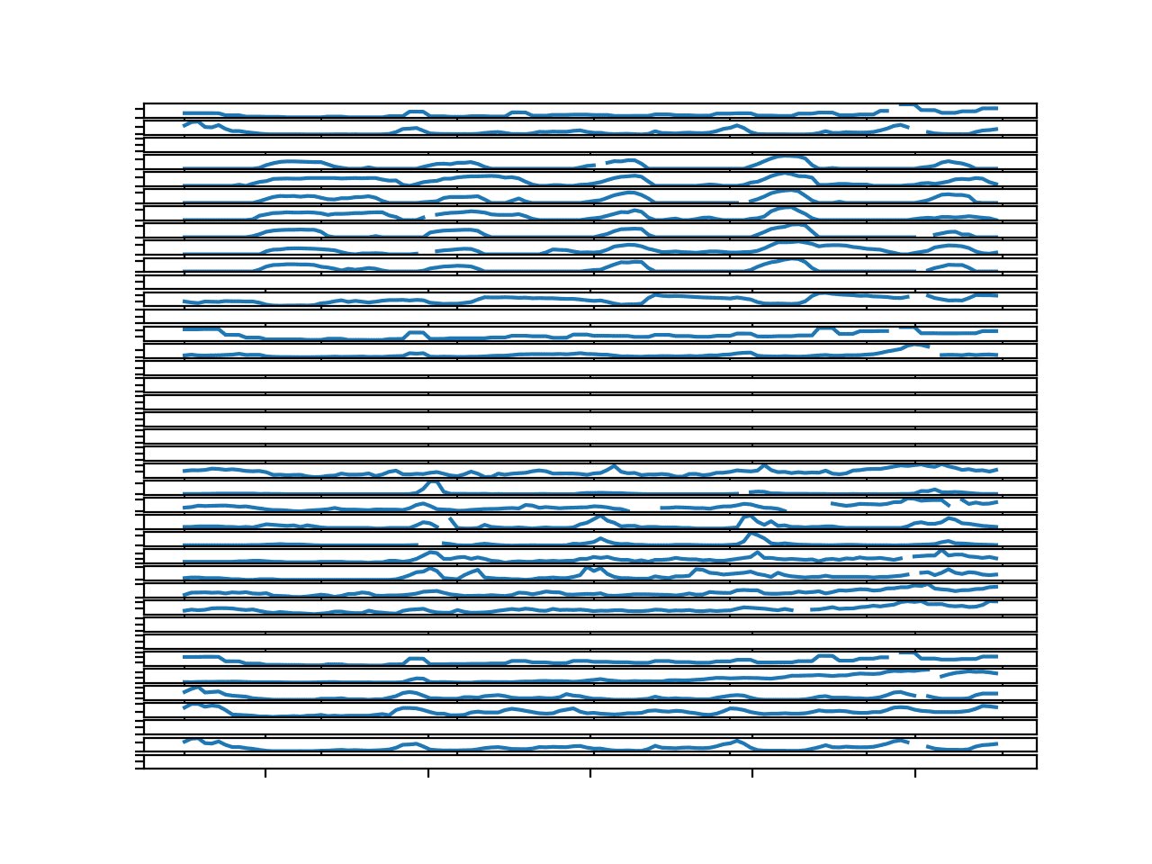
Running the example creates a figure with 39 line plots, one for each target variable in the first chunk.
We can see a seasonal structure in many of the variables. This suggests it may be beneficial to perform a 24-hour seasonal differencing of each series prior to modeling.
The plots are small, and you may need to increase the size of the figure to clearly see the data.
We can see that there are variables for which we have no data. These can be detected and ignored as we cannot model or forecast them.
We can see gaps in many of the series, but the gaps are short, lasting for a few hours at most. These could be imputed either with persistence of previous values or values at the same hours within the same series.
Line Plots for All Targets in Chunk 1 With Missing Values Marked
Looking at a few other chunks randomly, many result in plots with much the same observations.
This is not always the case though.
Update the example to plot the 4th chunk in the dataset (index 3).
1
2
# pick one chunk
rows=train_chunks[3]
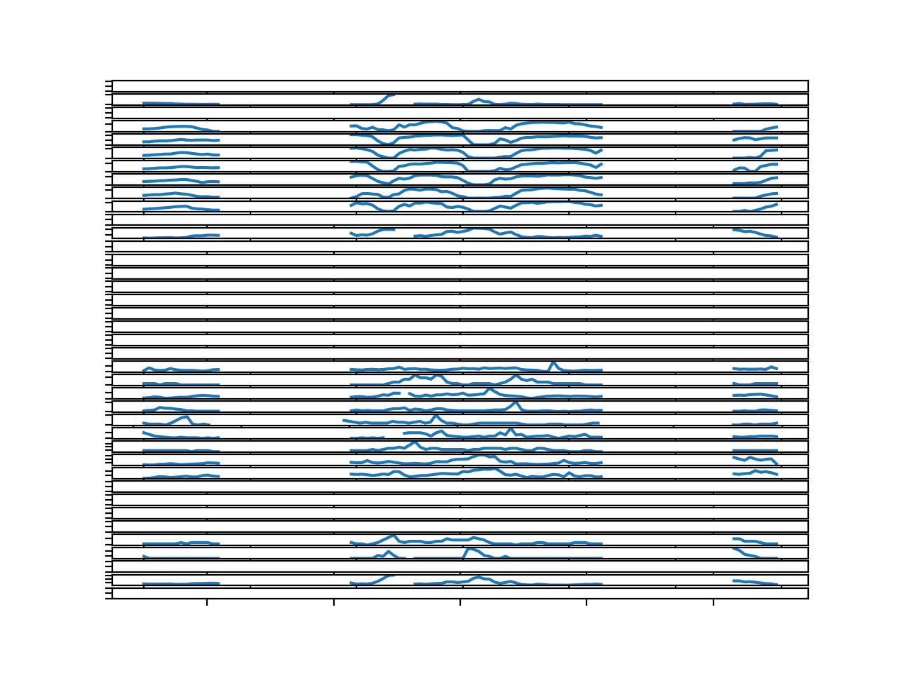
The result is a figure that tells a very different story.
We see gaps in the data that last for many hours, perhaps up to a day or more.
These series will require dramatic repair before they can be used to fit a classical model.
Imputing the missing data using persistence or observations within the series with the same hour will likely not be sufficient. They may have to be filled with average values taken across the entire training dataset.
Line Plots for All Targets in Chunk 4 With Missing Values Marked
Impute Missing Data
There are many ways to impute the missing data, and we cannot know which is best a priori.
One approach would be to prepare the data using multiple different imputation methods and use the skill of the models fit on the data to help guide the best approach.
Some imputation approaches already suggested include:
Persist the last observation in the series, also called linear interpolation.
Fill with values or average values within the series with the same hour of day.
Fill with values or average values with the same hour of day across the training dataset.
It may also be useful to use combinations, e.g. persist or fill from the series for small gaps and draw from the whole dataset for large gaps.
We can also investigate the effect of imputing methods by filling in the missing data and looking at plots to see if the series looks reasonable. It’s crude, effective, and fast.
First, we need to calculate a parallel series of the hour of day for each chunk that we can use for imputing hour-specific data for each variable in the chunk.
Given a series of partially filled hours of day, the interpolate_hours() function below will fill in the missing hours of day. It does this by finding the first marked hour, then counting forward, filling in the hour of day, then performing the same operation backwards.
1
2
3
4
5
6
7
8
9
10
11
12
13
14
15
16
17
18
19
20
21
22
23
24
# interpolate series of hours (in place) in 24 hour time
def interpolate_hours(hours):
# find the first hour
ix=-1
foriinrange(len(hours)):
ifnotisnan(hours[i]):
ix=i
break
# fill-forward
hour=hours[ix]
foriinrange(ix+1,len(hours)):
# increment hour
hour+=1
# check for a fill
ifisnan(hours[i]):
hours[i]=hour%24
# fill-backward
hour=hours[ix]
foriinrange(ix-1,-1,-1):
# decrement hour
hour-=1
# check for a fill
ifisnan(hours[i]):
hours[i]=hour%24
I’m sure there is a more Pythonic way to write this function, but I wanted to lay it all out to make it obvious what was going on.
We can test this out on a mock list of hours with missing data. The complete example is listed below.
1
2
3
4
5
6
7
8
9
10
11
12
13
14
15
16
17
18
19
20
21
22
23
24
25
26
27
28
29
30
31
32
33
34
35
# interpolate hours
from numpy import nan
from numpy import isnan
# interpolate series of hours (in place) in 24 hour time
We can use this function to prepare a series of hours for a chunk that can be used to fill in missing values for a chunk using hour-specific information.
We can call the same variable_to_series() function from the previous section to create the series of hours with missing values (column index 2), then call interpolate_hours() to fill in the gaps.
1
2
3
4
# prepare sequence of hours for the chunk
hours=variable_to_series(rows,2)
# interpolate hours
interpolate_hours(hours)
We can then pass the hours to any impute function that may make use of it.
Let’s try filling in missing values in a chunk with values within the same series with the same hour. Specifically, we will find all rows with the same hour on the series and calculate the median value.
The impute_missing() below takes all of the rows in a chunk, the prepared sequence of hours of the day for the chunk, and the series with missing values for a variable and the column index for a variable.
It first checks to see if the series is all missing data and returns immediately if this is the case as no impute can be performed. It then enumerates over the time steps of the series and when it detects a time step with no data, it collects all rows in the series with data for the same hour and calculates the median value.
1
2
3
4
5
6
7
8
9
10
11
12
13
14
15
16
17
18
19
20
21
# impute missing data
def impute_missing(rows,hours,series,col_ix):
# count missing observations
n_missing=count_nonzero(isnan(series))
# calculate ratio of missing
ratio=n_missing/float(len(series))*100
# check for no data
ifratio==100.0:
returnseries
# impute missing using the median value for hour in the series
imputed=list()
foriinrange(len(series)):
ifisnan(series[i]):
# get all rows with the same hour
matches=rows[rows[:,2]==hours[i]]
# fill with median value
value=nanmedian(matches[:,col_ix])
imputed.append(value)
else:
imputed.append(series[i])
returnimputed
To see the impact of this impute strategy, we can update the plot_variables() function from the previous section to first plot the imputed series then plot the original series with missing values.
This will allow the imputed values to shine through in the gaps of the original series and we can see if the results look reasonable.
The updated version of the plot_variables() function is listed below with this change, calling the impute_missing() function to create the imputed version of the series and taking the hours series as an argument.
1
2
3
4
5
6
7
8
9
10
11
12
13
14
15
16
17
18
19
# plot variables horizontally with gaps for missing data
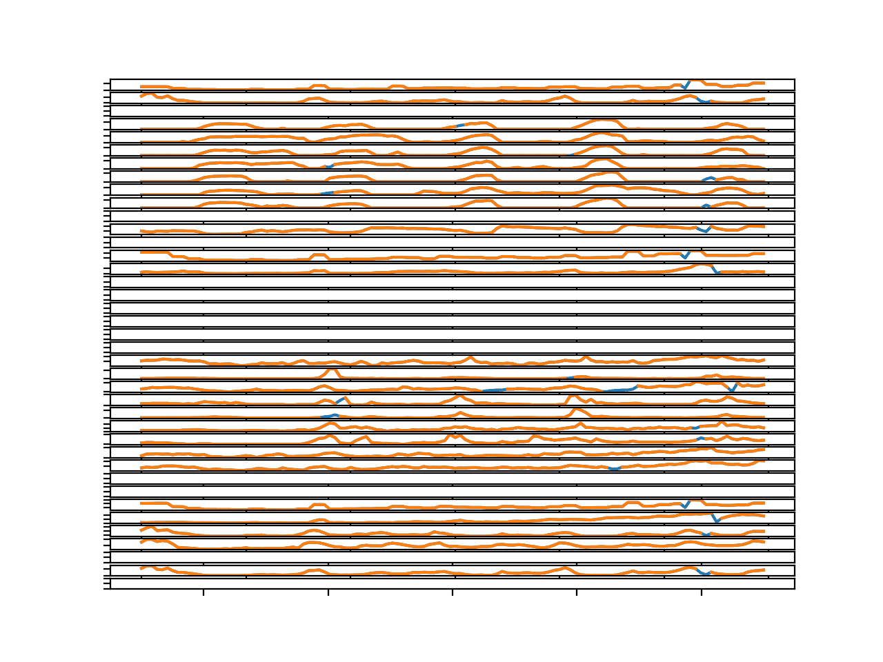
Running the example creates a single figure with 39 line plots: one for each target variable in the first chunk in the training dataset.
We can see that the series is orange, showing the original data and the gaps have been imputed and are marked in blue.
The blue segments seem reasonable.
Line Plots for All Targets in Chunk 1 With Imputed Missing Values
We can try the same approach on the 4th chunk in the dataset that has a lot more missing data.
1
2
# pick one chunk
rows=train_chunks[0]
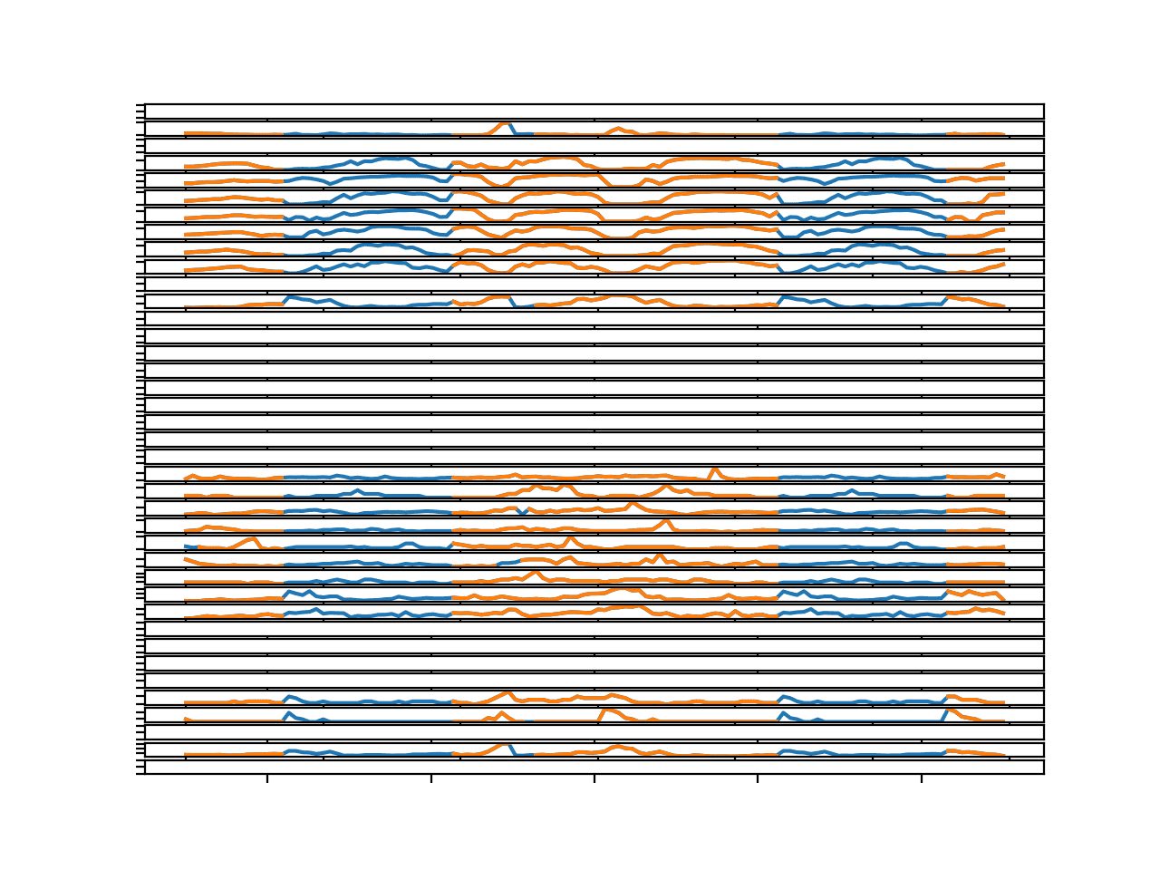
Running the example creates the same kind of figure, but here we can see the large missing segments filled in with imputed values.
Again, the sequences seem reasonable, even showing daily seasonal cycle structure where appropriate.
Line Plots for All Targets in Chunk 4 With Imputed Missing Values
This looks like a good start; you can explore other imputation strategies and see how they compare either in terms of line plots or on the resulting model skill.
Autocorrelation Plots
Now that we know how to fill in the missing values, we can take a look at autocorrelation plots for the series data.
Autocorrelation plots summarize the relationship of each observation with observations at prior time steps. Together with partial autocorrelation plots, they can be used to determine the configuration for an ARMA model.
The statsmodels library provides the plot_acf() and plot_pacf() functions that can be used to plot ACF and PACF plots respectively.
We can update the plot_variables() to create these plots, one of each type for each of the 39 series. That is a lot of plots.
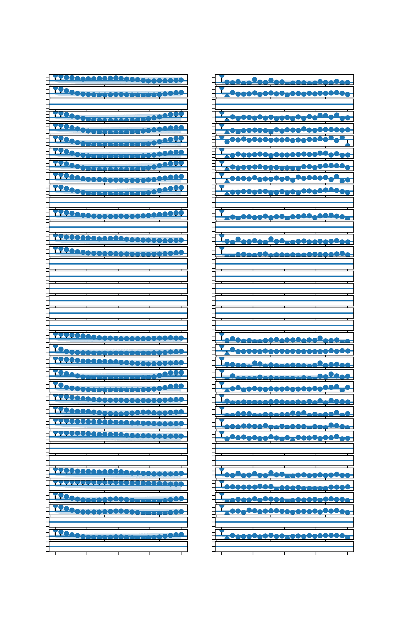
We will stack all ACF plots on the left vertically and all PACF plots on the right vertically. That is two columns of 39 plots. We will limit the lags considered by the plot to 24 time steps (hours) and ignore the correlation of each variable with itself as it is redundant.
The updated plot_variables() function for plotting ACF and PACF plots is listed below.
1
2
3
4
5
6
7
8
9
10
11
12
13
14
15
16
17
18
19
20
21
22
23
24
25
26
27
# plot acf and pacf plots for each imputed variable series
Running the example creates a figure with a lot of plots for the target variables in the first chunk of the training dataset.
You may need to increase the size of the plot window to better see the details of each plot.
We can see on the left that most ACF plots show significant correlations (dots above the significance region) at lags 1-2 steps, maybe lags 1-3 steps in some cases, with a slow, steady decrease over the lags
Similarly, on the right, we can see significant lags in the PACF plot at 1-2 time steps with steep fall-off.
This strongly suggests an autocorrelation process with an order of perhaps 1, 2, or 3, e.g. AR(3).
In the ACF plots on the left we can also see a daily cycle in the correlations. This may suggest some benefit in a seasonal differencing of the data prior to modeling or the use of an AR model capable of seasonal differencing.
ACF and PACF Plots for Target Variables in Chunk 1
We can repeat this analysis of the target variables for other chunks and we see much the same picture.
It suggests we may be able to get away with a general AR model configuration for all series across all chunks.
Develop an Autoregressive Model
In this section, we will develop an autoregressive model for the imputed target series data.
The first step is to implement a general function for making a forecast for each chunk.
The function tasks the training dataset and the input columns (chunk id, position in chunk, and hour) for the test set and returns forecasts for all chunks with the expected 3D format of [chunk][variable][time].
The function enumerates the chunks in the forecast, then enumerates the 39 target columns, calling another new function named forecast_variable() in order to make a prediction for each lead time for a given target variable.
The complete function is listed below.
1
2
3
4
5
6
7
8
9
10
11
12
13
14
15
16
17
18
# forecast for each chunk, returns [chunk][variable][time]
We can now implement a version of the forecast_variable().
For each variable, we first check if there is no data (e.g. all NaNs) and if so, we return a forecast that is a NaN for each forecast lead time.
We then create a series from the variable using the variable_to_series() and then impute the missing values using the median within the series by calling impute_missing(), both of which were developed in the previous section.
Finally, we call a new function named fit_and_forecast() that fits a model and predicts the 10 forecast lead times.
We will fit an AR model to a given imputed series. To do this, we will use the statsmodels ARIMA class. We will use ARIMA instead of AR to offer some flexibility if you would like to explore any of the family of ARIMA models.
First, we must define the model, including the order of the autoregressive process, such as AR(1).
1
2
# define the model
model=ARIMA(series,order=(1,0,0))
Next, the model is fit on the imputed series. We turn off the verbose information during the fit by setting disp to False.
1
2
# fit the model
model_fit=model.fit()
The fit model is then used to forecast the next 72 hours beyond the end of the series.
We are only interested in specific lead times, so we prepare an array of those lead times, subtract 1 to turn them into array indices, then use them to select the values at the 10 forecast lead times in which we are interested.
1
2
3
4
# extract lead times
lead_times=array(get_lead_times())
indices=lead_times-1
returnyhat[indices]
The statsmodels ARIMA models use linear algebra libraries to fit the model under the covers, and sometimes the fit process can be unstable on some data. As such, it can throw an exception or report a lot of warnings.
We will trap exceptions and return a NaN forecast, and ignore all warnings during the fit and evaluation.
The fit_and_forecast() function below ties all of this together.
Running the example first reports the overall MAE for the test set, followed by the MAE for each forecast lead time.
Note: Your results may vary given the stochastic nature of the algorithm or evaluation procedure, or differences in numerical precision. Consider running the example a few times and compare the average outcome.
We can see that the model achieves a MAE of about 0.492, which is less than a MAE 0.520 achieved by a naive persistence model. This shows that indeed the approach has some skill.
Re-running the example with the update shows an increase in the overall MAE compared to an AR(2).
An AR(2) might be a good global level configuration to use, although it is expected that models tailored to each variable or each series may perform better overall.
We can evaluate the AR(2) model with an alternate imputation strategy.
Instead of calculating the median value for the same hour across the series in the chunk, we can calculate the same value across the variable in all chunks.
We can update the impute_missing() to take all training chunks as an argument, then collect rows from all chunks for a given hour in order to calculate the median value used to impute. The updated version of the function is listed below.
In order to pass the train_chunks to the impute_missing() function, we must update the forecast_variable() function to also take train_chunks as an argument and pass it along, and in turn update the forecast_chunks() function to pass train_chunks.
The complete example using a global imputation strategy is listed below.
1
2
3
4
5
6
7
8
9
10
11
12
13
14
15
16
17
18
19
20
21
22
23
24
25
26
27
28
29
30
31
32
33
34
35
36
37
38
39
40
41
42
43
44
45
46
47
48
49
50
51
52
53
54
55
56
57
58
59
60
61
62
63
64
65
66
67
68
69
70
71
72
73
74
75
76
77
78
79
80
81
82
83
84
85
86
87
88
89
90
91
92
93
94
95
96
97
98
99
100
101
102
103
104
105
106
107
108
109
110
111
112
113
114
115
116
117
118
119
120
121
122
123
124
125
126
127
128
129
130
131
132
133
134
135
136
137
138
139
140
141
142
143
144
145
146
147
148
149
150
151
152
153
154
155
156
157
158
159
160
161
162
163
164
165
166
167
168
169
170
171
172
173
174
175
176
177
178
179
180
181
182
183
184
185
186
187
188
189
190
191
192
193
194
195
196
197
198
199
200
201
202
203
204
205
206
207
208
209
210
211
212
213
214
215
216
217
218
219
220
221
# autoregression forecast with global impute strategy
from numpy import loadtxt
from numpy import nan
from numpy import isnan
from numpy import count_nonzero
from numpy import unique
from numpy import array
from numpy import nanmedian
from statsmodels.tsa.arima.model import ARIMA
from matplotlib import pyplot
from warnings import catch_warnings
from warnings import filterwarnings
# split the dataset by 'chunkID', return a list of chunks
def to_chunks(values,chunk_ix=0):
chunks=list()
# get the unique chunk ids
chunk_ids=unique(values[:,chunk_ix])
# group rows by chunk id
forchunk_id inchunk_ids:
selection=values[:,chunk_ix]==chunk_id
chunks.append(values[selection,:])
returnchunks
# return a list of relative forecast lead times
def get_lead_times():
return[1,2,3,4,5,10,17,24,48,72]
# interpolate series of hours (in place) in 24 hour time
Note: Your results may vary given the stochastic nature of the algorithm or evaluation procedure, or differences in numerical precision. Consider running the example a few times and compare the average outcome.
Running the example shows a further drop in the overall MAE to about 0.487.
It may be interesting to explore imputation strategies that alternate the method used to fill in missing values based on how much missing data a series has or the gap being filled.
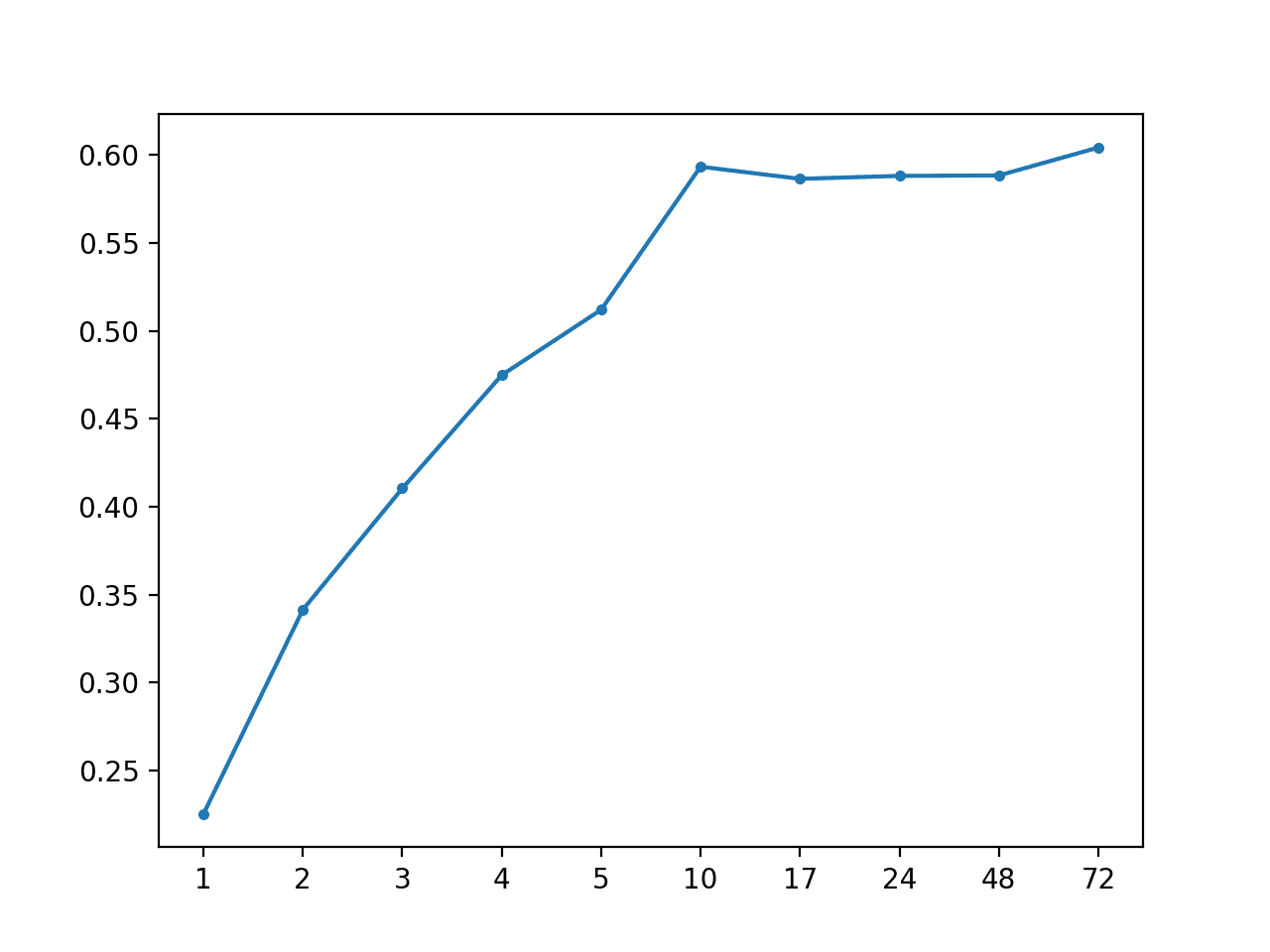
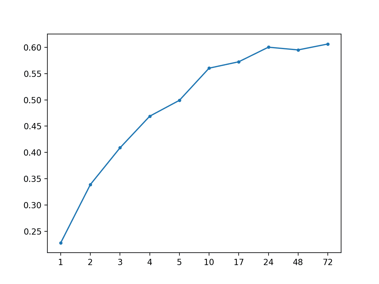
A line plot of MAE vs. forecast lead time is also created.
MAE vs Forecast Lead Time for AR(2) Impute With Global Strategy
Extensions
This section lists some ideas for extending the tutorial that you may wish to explore.
Imputation Strategies. Develop and evaluate one additional alternate imputation strategy for the missing data in each series.
Data Preparation. Explore whether data preparation techniques applied to each can improve model skill, such as standardization, normalization, and power transforms.
Differencing. Explore whether differencing, such as 1-step or 24-step (seasonal differencing), can make each series stationary, and in turn result in better forecasts.
If you explore any of these extensions, I’d love to know.
Further Reading
This section provides more resources on the topic if you are looking to go deeper.
In this tutorial, you discovered how to develop autoregressive models for multi-step time series forecasting for a multivariate air pollution time series.
Specifically, you learned:
How to analyze and impute missing values for time series data.
How to develop and evaluate an autoregressive model for multi-step time series forecasting.
How to improve an autoregressive model using alternate data imputation methods.
Do you have any questions?
Ask your questions in the comments below and I will do my best to answer.
Develop Deep Learning models for Time Series Today!
Hi Dr. Brownlee! Awesome job done as always! Thank you so much for your contribution.
I wonder is it possible to implement some kind of Machine Learning methods to fill missing data by neighboring stations. I mean if there are several stations with correlated observed timeseries and I want to use them to fill missing timeseries data in the station that I use for modeling. Usually pairwise correlation method used for such tasks and it is statistically based approach, maybe it would be better to use Neural Networks. What do you think? Thanks.
Thank you for sharing the above interesting analysis.
However, i was wondering if it is possible to find the best ARIMA model for each site/location instead of each chuch, since we have data (target/variables) for few sites.
For this approach can we use the meteorological data for finding a correlation between sites?
Any suggestions? Thank you in advance!
Hi Jason,
If i understand well, in this tutorial you forecast each of the variables (wind speed, temperature..) and then the air quality is a function of the outputs obtained ? In otherwords, we do not fit an arima model that would integrate all these exogenous factors to predict the air quality ?
I am asking as this is precisely what i am trying to do with a time series of electrical load and one of temperature. My goal is to forecast the electrical load while taking into account its dependence on the outdoor temperature. So i am using a sarimax model with the temperature time series as an exogenous variable, and doing a grid search to obtain the best model. But then i am facing different issues:
– the sarimax model only provides one coefficient for temperature, like a linear regression. Given the existence of inertia in the load response to temperature, i would ideally want to have a autoregressive model not only on the load itself but on temperature. That is, integrating the temperature T at time t, but also lags of temperature. Would you know if it could be possible to achieve that with a sarimax, for exemple by having multiple exogenous regressors ? Or should i ultimately try another model, like LTSM ? The same question applies if i wanted to integrate other data like wind speed or solar radiation to improve the accuracy of the load forecast.
– i have 10 years of hourly data, and use only the winter period. my ultimate goal is to forecast a year of load and derive specifically the peak load. So i would need to use different years as part of the training data, and test on one year / a part of a year. Would you have a recommendation on how to make sure that the discontinuous period between march and november of year x does not ruin the forecasts ?
– my last question is related to the trend i have in the data, as the consumption has globally increased (not linearly) across years. However this is a slow trend that cannot be observed within a year of observations, especially as the load varies mostly with the outdoor temperature.( For instance, a ‘warm’ winter will have low loads and a ‘cold’ winter will have a higher level so this trend is hard to observe across years). Therefore, i am planning to train the data only on a limited number of consecutive years to limit that effect, but at the same time i would need to integrate this trend in my model in order to make an accurate forecast for the future. How could i do it, and make sure that i do not obtain a model that does not represent the real evolution if i do not train it on the most recent years only ?
I hope my questions are clear, and i thank you so much in advance for your help. I have been reading your articles for several months and do most of the time find my answers in the comments already adressed, but these i haven’t:)


Hi Dr. Brownlee! Awesome job done as always! Thank you so much for your contribution.
I wonder is it possible to implement some kind of Machine Learning methods to fill missing data by neighboring stations. I mean if there are several stations with correlated observed timeseries and I want to use them to fill missing timeseries data in the station that I use for modeling. Usually pairwise correlation method used for such tasks and it is statistically based approach, maybe it would be better to use Neural Networks. What do you think? Thanks.
Sure, try it and let me know how you go.
Thank you for sharing the above interesting analysis.
However, i was wondering if it is possible to find the best ARIMA model for each site/location instead of each chuch, since we have data (target/variables) for few sites.
For this approach can we use the meteorological data for finding a correlation between sites?
Any suggestions? Thank you in advance!
Perhaps try it and see.
Hi,
I wonder how to do the same in R?
Sorry, I don’t have examples in R.
Thank you for sharing the above interesting analysis
why my one step result differs from the first step result of my multi-step results?
Because there are some randomness in training the machine learning models, hence the models trained are not always match.
Hi Jason,
If i understand well, in this tutorial you forecast each of the variables (wind speed, temperature..) and then the air quality is a function of the outputs obtained ? In otherwords, we do not fit an arima model that would integrate all these exogenous factors to predict the air quality ?
I am asking as this is precisely what i am trying to do with a time series of electrical load and one of temperature. My goal is to forecast the electrical load while taking into account its dependence on the outdoor temperature. So i am using a sarimax model with the temperature time series as an exogenous variable, and doing a grid search to obtain the best model. But then i am facing different issues:
– the sarimax model only provides one coefficient for temperature, like a linear regression. Given the existence of inertia in the load response to temperature, i would ideally want to have a autoregressive model not only on the load itself but on temperature. That is, integrating the temperature T at time t, but also lags of temperature. Would you know if it could be possible to achieve that with a sarimax, for exemple by having multiple exogenous regressors ? Or should i ultimately try another model, like LTSM ? The same question applies if i wanted to integrate other data like wind speed or solar radiation to improve the accuracy of the load forecast.
– i have 10 years of hourly data, and use only the winter period. my ultimate goal is to forecast a year of load and derive specifically the peak load. So i would need to use different years as part of the training data, and test on one year / a part of a year. Would you have a recommendation on how to make sure that the discontinuous period between march and november of year x does not ruin the forecasts ?
– my last question is related to the trend i have in the data, as the consumption has globally increased (not linearly) across years. However this is a slow trend that cannot be observed within a year of observations, especially as the load varies mostly with the outdoor temperature.( For instance, a ‘warm’ winter will have low loads and a ‘cold’ winter will have a higher level so this trend is hard to observe across years). Therefore, i am planning to train the data only on a limited number of consecutive years to limit that effect, but at the same time i would need to integrate this trend in my model in order to make an accurate forecast for the future. How could i do it, and make sure that i do not obtain a model that does not represent the real evolution if i do not train it on the most recent years only ?
I hope my questions are clear, and i thank you so much in advance for your help. I have been reading your articles for several months and do most of the time find my answers in the comments already adressed, but these i haven’t:)
Kind regards,
Magali
Hi Magali,
While I cannot speak to your specific application, I would highly recommend that you investigate a multivariate LSTM model.
https://machinelearningmastery.com/multivariate-time-series-forecasting-lstms-keras/