What Is a Gradient in Machine Learning?

Gradient is a commonly used term in optimization and machine learning.

For example, deep learning neural networks are fit using stochastic gradient descent, and many standard optimization algorithms used to fit machine learning algorithms use gradient information.

In order to understand what a gradient is, you need to understand what a derivative is from the field of calculus. This includes how to calculate a derivative and interpret the value. An understanding of the derivative is directly applicable to understanding how to calculate and interpret gradients as used in optimization and machine learning.

In this tutorial, you will discover a gentle introduction to the derivative and the gradient in machine learning.

After completing this tutorial, you will know:

• The derivative of a function is the change of the function for a given input.
• The gradient is simply a derivative vector for a multivariate function.
• How to calculate and interpret derivatives of a simple function.

Kick-start your project with my new book Optimization for Machine Learning, including step-by-step tutorials and the Python source code files for all examples.

What Is a Gradient in Machine Learning?
Photo by Roanish, some rights reserved.

Tutorial Overview

This tutorial is divided into five parts; they are:

1. What Is a Derivative?
2. What Is a Gradient?
3. Worked Example of Calculating Derivatives
4. How to Interpret the Derivative
5. How to Calculate a the Derivative of a Function

What Is a Derivative?

In calculus, a derivative is the rate of change at a given point in a real-valued function.

For example, the derivative f'(x) of function f() for variable x is the rate that the function f() changes at the point x.

It might change a lot, e.g. be very curved, or might change a little, e.g. slight curve, or it might not change at all, e.g. flat or stationary.

A function is differentiable if we can calculate the derivative at all points of input for the function variables. Not all functions are differentiable.

Once we calculate the derivative, we can use it in a number of ways.

For example, given an input value x and the derivative at that point f'(x), we can estimate the value of the function f(x) at a nearby point delta_x (change in x) using the derivative, as follows:

• f(x + delta_x) = f(x) + f'(x) * delta_x

Here, we can see that f'(x) is a line and we are estimating the value of the function at a nearby point by moving along the line by delta_x.

We can use derivatives in optimization problems as they tell us how to change inputs to the target function in a way that increases or decreases the output of the function, so we can get closer to the minimum or maximum of the function.

Derivatives are useful in optimization because they provide information about how to change a given point in order to improve the objective function.

— Page 32, Algorithms for Optimization, 2019.

Finding the line that can be used to approximate nearby values was the main reason for the initial development of differentiation. This line is referred to as the tangent line or the slope of the function at a given point.

The problem of finding the tangent line to a curve […] involve finding the same type of limit […] This special type of limit is called a derivative and we will see that it can be interpreted as a rate of change in any of the sciences or engineering.

— Page 104, Calculus, 8th edition, 2015.

An example of the tangent line of a point for a function is provided below, taken from page 19 of “Algorithms for Optimization.”

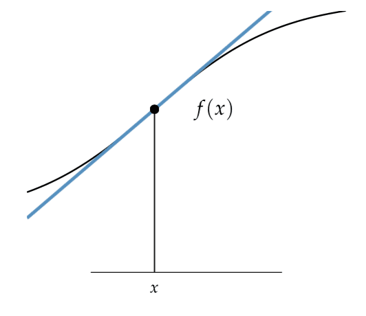
Tangent Line of a Function at a Given Point
Taken from Algorithms for Optimization.

Technically, the derivative described so far is called the first derivative or first-order derivative.

The second derivative (or second-order derivative) is the derivative of the derivative function. That is, the rate of change of the rate of change or how much the change in the function changes.

• First Derivative: Rate of change of the target function.
• Second Derivative: Rate of change of the first derivative function.

A natural use of the second derivative is to approximate the first derivative at a nearby point, just as we can use the first derivative to estimate the value of the target function at a nearby point.

Now that we know what a derivative is, let’s take a look at a gradient.

What Is a Gradient?

A gradient is a derivative of a function that has more than one input variable.

It is a term used to refer to the derivative of a function from the perspective of the field of linear algebra. Specifically when linear algebra meets calculus, called vector calculus.

The gradient is the generalization of the derivative to multivariate functions. It captures the local slope of the function, allowing us to predict the effect of taking a small step from a point in any direction.

— Page 21, Algorithms for Optimization, 2019.

Multiple input variables together define a vector of values, e.g. a point in the input space that can be provided to the target function.

The derivative of a target function with a vector of input variables similarly is a vector. This vector of derivatives for each input variable is the gradient.

• Gradient (vector calculus): A vector of derivatives for a function that takes a vector of input variables.

You might recall from high school algebra or pre-calculus, the gradient also refers generally to the slope of a line on a two-dimensional plot.

It is calculated as the rise (change on the y-axis) of the function divided by the run (change in x-axis) of the function, simplified to the rule: “rise over run“:

• Gradient (algebra): Slope of a line, calculated as rise over run.

We can see that this is a simple and rough approximation of the derivative for a function with one variable. The derivative function from calculus is more precise as it uses limits to find the exact slope of the function at a point. This idea of gradient from algebra is related, but not directly useful to the idea of a gradient as used in optimization and machine learning.

A function that takes multiple input variables, e.g. a vector of input variables, may be referred to as a multivariate function.

The partial derivative of a function with respect to a variable is the derivative assuming all other input variables are held constant.

— Page 21, Algorithms for Optimization, 2019.

Each component in the gradient (vector of derivatives) is called a partial derivative of the target function.

A partial derivative assumes all other variables of the function are held constant.

• Partial Derivative: A derivative for one of the variables for a multivariate function.

It is useful to work with square matrices in linear algebra, and the square matrix of the second-order derivatives is referred to as the Hessian matrix.

The Hessian of a multivariate function is a matrix containing all of the second derivatives with respect to the input

— Page 21, Algorithms for Optimization, 2019.

We can use gradient and derivative interchangeably, although in the fields of optimization and machine learning, we typically use “gradient” as we are typically concerned with multivariate functions.

Intuitions for the derivative translate directly to the gradient, only with more dimensions.

Now that we are familiar with the idea of a derivative and a gradient, let’s look at a worked example of calculating derivatives.

Worked Example of Calculating Derivatives

Let’s make the derivative concrete with a worked example.

First, let’s define a simple one-dimensional function that squares the input and defines the range of valid inputs from -1.0 to 1.0.

• f(x) = x^2

The example below samples inputs from this function in 0.1 increments, calculates the function value for each input, and plots the result.

Running the example creates a line plot of the inputs to the function (x-axis) and the calculated output of the function (y-axis).

We can see the familiar U-shaped called a parabola.

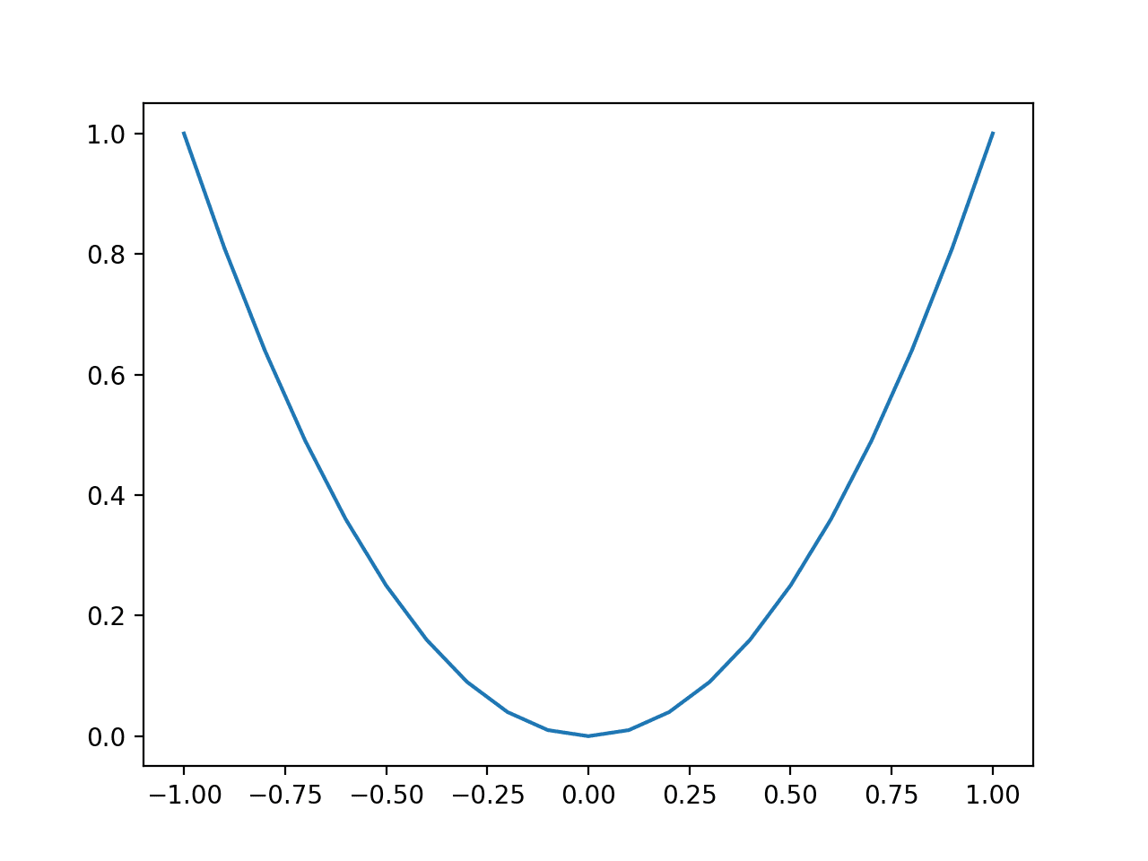
Line Plot of Simple One Dimensional Function

We can see a large change or steep curve on the sides of the shape where we would expect a large derivative and a flat area in the middle of the function where we would expect a small derivative.

Let’s confirm these expectations by calculating the derivative at -0.5 and 0.5 (steep) and 0.0 (flat).

The derivative for the function is calculated as follows:

• f'(x) = x * 2

The example below calculates the derivatives for the specific input points for our objective function.

Running the example prints the derivative values for specific input values.

We can see that the derivative at the steep points of the function is -1 and 1 and the derivative for the flat part of the function is 0.0.

Now that we know how to calculate derivatives of a function, let’s look at how we might interpret the derivative values.

How to Interpret the Derivative

The value of the derivative can be interpreted as the rate of change (magnitude) and the direction (sign).

• Magnitude of Derivative: How much change.
• Sign of Derivative: Direction of change.

A derivative of 0.0 indicates no change in the target function, referred to as a stationary point.

A function may have one or more stationary points and a local or global minimum (bottom of a valley) or maximum (peak of a mountain) of the function are examples of stationary points.

The gradient points in the direction of steepest ascent of the tangent hyperplane …

— Page 21, Algorithms for Optimization, 2019.

The sign of the derivative tells you if the target function is increasing or decreasing at that point.

• Positive Derivative: Function is increasing at that point.
• Negative Derivative: Function is decreasing at that point

This might be confusing because, looking at the plot from the previous section, the values of the function f(x) are increasing on the y-axis for -0.5 and 0.5.

The trick here is to always read the plot of the function from left to right, e.g. follow the values on the y-axis from left to right for input x-values.

Indeed the values around x=-0.5 are decreasing if read from left to right, hence the negative derivative, and the values around x=0.5 are increasing, hence the positive derivative.

We can imagine that if we wanted to find the minima of the function in the previous section using only the gradient information, we would increase the x input value if the gradient was negative to go downhill, or decrease the value of x input if the gradient was positive to go downhill.

This is the basis for the gradient descent (and gradient ascent) class of optimization algorithms that have access to function gradient information.

Now that we know how to interpret derivative values, let’s look at how we might find the derivative of a function.

How to Calculate a the Derivative of a Function

Finding the derivative function f'() that outputs the rate of change of a target function f() is called differentiation.

There are many approaches (algorithms) for calculating the derivative of a function.

In some cases, we can calculate the derivative of a function using the tools of calculus, either manually or using an automatic solver.

General classes of techniques for calculating the derivative of a function include:

• Finite difference method
• Symbolic differentiation
• Automatic differentiation

The SymPy Python library can be used for symbolic differentiation.

Computational libraries such as Theano and TensorFlow can be used for automatic differentiation.

There are also online services you can use if your function is easy to specify in plain text.

One example is the Wolfram Alpha website that will calculate the derivative of the function for you; for example:

• Calculate the Derivative of x^2

Not all functions are differentiable, and some functions that are differentiable may make it difficult to find the derivative with some methods.

Calculating the derivative of a function is beyond the scope of this tutorial. Consult a good calculus textbook, such as those in the further reading section.

Further Reading

This section provides more resources on the topic if you are looking to go deeper.

Books

• Algorithms for Optimization, 2019.
• Calculus, 3rd Edition, 2017. (Gilbert Strang)
• Calculus, 8th edition, 2015. (James Stewart)

Articles

• Derivative, Wikipedia.
• Second derivative, Wikipedia.
• Partial derivative, Wikipedia.
• Gradient, Wikipedia.
• Differentiable function, Wikipedia.
• Jacobian matrix and determinant, Wikipedia.
• Hessian matrix, Wikipedia.

Summary

In this tutorial, you discovered a gentle introduction to the derivative and the gradient in machine learning.

Specifically, you learned:

• The derivative of a function is the change of the function for a given input.
• The gradient is simply a derivative vector for a multivariate function.
• How to calculate and interpret derivatives of a simple function.

Do you have any questions?
Ask your questions in the comments below and I will do my best to answer.

Get a Handle on Modern Optimization Algorithms!

Develop Your Understanding of Optimization

...with just a few lines of python code

Discover how in my new Ebook:
Optimization for Machine Learning

It provides self-study tutorials with full working code on:
Gradient Descent, Genetic Algorithms, Hill Climbing, Curve Fitting, RMSProp, Adam, and much more...

Bring Modern Optimization Algorithms to
Your Machine Learning Projects

See What's Inside