
The Gradient Boosting Machine is a powerful ensemble machine learning algorithm that uses decision trees.
Boosting is a general ensemble technique that involves sequentially adding models to the ensemble where subsequent models correct the performance of prior models. AdaBoost was the first algorithm to deliver on the promise of boosting.
Gradient boosting is a generalization of AdaBoosting, improving the performance of the approach and introducing ideas from bootstrap aggregation to further improve the models, such as randomly sampling the samples and features when fitting ensemble members.
Gradient boosting performs well, if not the best, on a wide range of tabular datasets, and versions of the algorithm like XGBoost and LightBoost often play an important role in winning machine learning competitions.
In this tutorial, you will discover how to develop Gradient Boosting ensembles for classification and regression.
After completing this tutorial, you will know:
- Gradient Boosting ensemble is an ensemble created from decision trees added sequentially to the model.
- How to use the Gradient Boosting ensemble for classification and regression with scikit-learn.
- How to explore the effect of Gradient Boosting model hyperparameters on model performance.
Kick-start your project with my new book Ensemble Learning Algorithms With Python, including step-by-step tutorials and the Python source code files for all examples.
Let’s get started.
- Update Aug/2020: Added a common questions section. Added grid search example.

How to Develop a Gradient Boosting Machine Ensemble in Python
Photo by Susanne Nilsson, some rights reserved.
Tutorial Overview
This tutorial is divided into five parts; they are:
- Gradient Boosting Algorithm
- Gradient Boosting Scikit-Learn API
- Gradient Boosting for Classification
- Gradient Boosting for Regression
- Gradient Boosting Hyperparameters
- Explore Number of Trees
- Explore Number of Samples
- Explore Number of Features
- Explore Learning Rate
- Explore Tree Depth
- Grid Search Hyperparameters
- Common Questions
Gradient Boosting Machines Algorithm
Gradient boosting refers to a class of ensemble machine learning algorithms that can be used for classification or regression predictive modeling problems.
Gradient boosting is also known as gradient tree boosting, stochastic gradient boosting (an extension), and gradient boosting machines, or GBM for short.
Ensembles are constructed from decision tree models. Trees are added one at a time to the ensemble and fit to correct the prediction errors made by prior models. This is a type of ensemble machine learning model referred to as boosting.
Models are fit using any arbitrary differentiable loss function and gradient descent optimization algorithm. This gives the technique its name, “gradient boosting,” as the loss gradient is minimized as the model is fit, much like a neural network.
One way to produce a weighted combination of classifiers which optimizes [the cost] is by gradient descent in function space
— Boosting Algorithms as Gradient Descent in Function Space, 1999.
Naive gradient boosting is a greedy algorithm and can overfit the training dataset quickly.
It can benefit from regularization methods that penalize various parts of the algorithm and generally improve the performance of the algorithm by reducing overfitting.
There are three types of enhancements to basic gradient boosting that can improve performance:
- Tree Constraints: such as the depth of the trees and the number of trees used in the ensemble.
- Weighted Updates: such as a learning rate used to limit how much each tree contributes to the ensemble.
- Random sampling: such as fitting trees on random subsets of features and samples.
The use of random sampling often leads to a change in the name of the algorithm to “stochastic gradient boosting.”
… at each iteration a subsample of the training data is drawn at random (without replacement) from the full training dataset. The randomly selected subsample is then used, instead of the full sample, to fit the base learner.
— Stochastic Gradient Boosting, 1999.
Gradient boosting is an effective machine learning algorithm and is often the main, or one of the main, algorithms used to win machine learning competitions (like Kaggle) on tabular and similar structured datasets.
For more on the gradient boosting algorithm, see the tutorial:
Now that we are familiar with the gradient boosting algorithm, let’s look at how we can fit GBM models in Python.
Want to Get Started With Ensemble Learning?
Take my free 7-day email crash course now (with sample code).
Click to sign-up and also get a free PDF Ebook version of the course.
Gradient Boosting Scikit-Learn API
Gradient Boosting ensembles can be implemented from scratch although can be challenging for beginners.
The scikit-learn Python machine learning library provides an implementation of Gradient Boosting ensembles for machine learning.
The algorithm is available in a modern version of the library.
First, confirm that you are using a modern version of the library by running the following script:
|
1 2 3 |
# check scikit-learn version import sklearn print(sklearn.__version__) |
Running the script will print your version of scikit-learn.
Your version should be the same or higher. If not, you must upgrade your version of the scikit-learn library.
|
1 |
0.22.1 |
Gradient boosting is provided via the GradientBoostingRegressor and GradientBoostingClassifier classes.
Both models operate the same way and take the same arguments that influence how the decision trees are created and added to the ensemble.
Randomness is used in the construction of the model. This means that each time the algorithm is run on the same data, it will produce a slightly different model.
When using machine learning algorithms that have a stochastic learning algorithm, it is good practice to evaluate them by averaging their performance across multiple runs or repeats of cross-validation. When fitting a final model, it may be desirable to either increase the number of trees until the variance of the model is reduced across repeated evaluations, or to fit multiple final models and average their predictions.
Let’s take a look at how to develop a Gradient Boosting ensemble for both classification and regression.
Gradient Boosting for Classification
In this section, we will look at using Gradient Boosting for a classification problem.
First, we can use the make_classification() function to create a synthetic binary classification problem with 1,000 examples and 20 input features.
The complete example is listed below.
|
1 2 3 4 5 6 |
# test classification dataset from sklearn.datasets import make_classification # define dataset X, y = make_classification(n_samples=1000, n_features=20, n_informative=15, n_redundant=5, random_state=7) # summarize the dataset print(X.shape, y.shape) |
Running the example creates the dataset and summarizes the shape of the input and output components.
|
1 |
(1000, 20) (1000,) |
Next, we can evaluate a Gradient Boosting algorithm on this dataset.
We will evaluate the model using repeated stratified k-fold cross-validation, with three repeats and 10 folds. We will report the mean and standard deviation of the accuracy of the model across all repeats and folds.
|
1 2 3 4 5 6 7 8 9 10 11 12 13 14 15 16 17 |
# evaluate gradient boosting algorithm for classification from numpy import mean from numpy import std from sklearn.datasets import make_classification from sklearn.model_selection import cross_val_score from sklearn.model_selection import RepeatedStratifiedKFold from sklearn.ensemble import GradientBoostingClassifier # define dataset X, y = make_classification(n_samples=1000, n_features=20, n_informative=15, n_redundant=5, random_state=7) # define the model model = GradientBoostingClassifier() # define the evaluation method cv = RepeatedStratifiedKFold(n_splits=10, n_repeats=3, random_state=1) # evaluate the model on the dataset n_scores = cross_val_score(model, X, y, scoring='accuracy', cv=cv, n_jobs=-1) # report performance print('Mean Accuracy: %.3f (%.3f)' % (mean(n_scores), std(n_scores))) |
Running the example reports the mean and standard deviation accuracy of the model.
Note: Your results may vary given the stochastic nature of the algorithm or evaluation procedure, or differences in numerical precision. Consider running the example a few times and compare the average outcome.
In this case, we can see the Gradient Boosting ensemble with default hyperparameters achieves a classification accuracy of about 89.9 percent on this test dataset.
|
1 |
Mean Accuracy: 0.899 (0.030) |
We can also use the Gradient Boosting model as a final model and make predictions for classification.
First, the Gradient Boosting ensemble is fit on all available data, then the predict() function can be called to make predictions on new data.
The example below demonstrates this on our binary classification dataset.
|
1 2 3 4 5 6 7 8 9 10 11 12 13 14 |
# make predictions using gradient boosting for classification from sklearn.datasets import make_classification from sklearn.ensemble import GradientBoostingClassifier # define dataset X, y = make_classification(n_samples=1000, n_features=20, n_informative=15, n_redundant=5, random_state=7) # define the model model = GradientBoostingClassifier() # fit the model on the whole dataset model.fit(X, y) # make a single prediction row = [0.2929949, -4.21223056, -1.288332, -2.17849815, -0.64527665, 2.58097719, 0.28422388, -7.1827928, -1.91211104, 2.73729512, 0.81395695, 3.96973717, -2.66939799, 3.34692332, 4.19791821, 0.99990998, -0.30201875, -4.43170633, -2.82646737, 0.44916808] yhat = model.predict([row]) # summarize prediction print('Predicted Class: %d' % yhat[0]) |
Running the example fits the Gradient Boosting ensemble model on the entire dataset and is then used to make a prediction on a new row of data, as we might when using the model in an application.
|
1 |
Predicted Class: 1 |
Now that we are familiar with using Gradient Boosting for classification, let’s look at the API for regression.
Gradient Boosting for Regression
In this section, we will look at using Gradient Boosting for a regression problem.
First, we can use the make_regression() function to create a synthetic regression problem with 1,000 examples and 20 input features.
The complete example is listed below.
|
1 2 3 4 5 6 |
# test regression dataset from sklearn.datasets import make_regression # define dataset X, y = make_regression(n_samples=1000, n_features=20, n_informative=15, noise=0.1, random_state=7) # summarize the dataset print(X.shape, y.shape) |
Running the example creates the dataset and summarizes the shape of the input and output components.
|
1 |
(1000, 20) (1000,) |
Next, we can evaluate a Gradient Boosting algorithm on this dataset.
As we did with the last section, we will evaluate the model using repeated k-fold cross-validation, with three repeats and 10 folds. We will report the mean absolute error (MAE) of the model across all repeats and folds. The scikit-learn library makes the MAE negative so that it is maximized instead of minimized. This means that larger negative MAE are better and a perfect model has a MAE of 0.
The complete example is listed below.
|
1 2 3 4 5 6 7 8 9 10 11 12 13 14 15 16 17 |
# evaluate gradient boosting ensemble for regression from numpy import mean from numpy import std from sklearn.datasets import make_regression from sklearn.model_selection import cross_val_score from sklearn.model_selection import RepeatedKFold from sklearn.ensemble import GradientBoostingRegressor # define dataset X, y = make_regression(n_samples=1000, n_features=20, n_informative=15, noise=0.1, random_state=7) # define the model model = GradientBoostingRegressor() # define the evaluation procedure cv = RepeatedKFold(n_splits=10, n_repeats=3, random_state=1) # evaluate the model n_scores = cross_val_score(model, X, y, scoring='neg_mean_absolute_error', cv=cv, n_jobs=-1) # report performance print('MAE: %.3f (%.3f)' % (mean(n_scores), std(n_scores))) |
Running the example reports the mean and standard deviation accuracy of the model.
Note: Your results may vary given the stochastic nature of the algorithm or evaluation procedure, or differences in numerical precision. Consider running the example a few times and compare the average outcome.
In this case, we can see the Gradient Boosting ensemble with default hyperparameters achieves a MAE of about 62.
|
1 |
MAE: -62.475 (3.254) |
We can also use the Gradient Boosting model as a final model and make predictions for regression.
First, the Gradient Boosting ensemble is fit on all available data, then the predict() function can be called to make predictions on new data.
The example below demonstrates this on our regression dataset.
|
1 2 3 4 5 6 7 8 9 10 11 12 13 14 |
# gradient boosting ensemble for making predictions for regression from sklearn.datasets import make_regression from sklearn.ensemble import GradientBoostingRegressor # define dataset X, y = make_regression(n_samples=1000, n_features=20, n_informative=15, noise=0.1, random_state=7) # define the model model = GradientBoostingRegressor() # fit the model on the whole dataset model.fit(X, y) # make a single prediction row = [0.20543991, -0.97049844, -0.81403429, -0.23842689, -0.60704084, -0.48541492, 0.53113006, 2.01834338, -0.90745243, -1.85859731, -1.02334791, -0.6877744, 0.60984819, -0.70630121, -1.29161497, 1.32385441, 1.42150747, 1.26567231, 2.56569098, -0.11154792] yhat = model.predict([row]) # summarize prediction print('Prediction: %d' % yhat[0]) |
Running the example fits the Gradient Boosting ensemble model on the entire dataset and is then used to make a prediction on a new row of data, as we might when using the model in an application.
|
1 |
Prediction: 37 |
Now that we are familiar with using the scikit-learn API to evaluate and use Gradient Boosting ensembles, let’s look at configuring the model.
Gradient Boosting Hyperparameters
In this section, we will take a closer look at some of the hyperparameters you should consider tuning for the Gradient Boosting ensemble and their effect on model performance.
There are perhaps four key hyperparameters that have the biggest effect on model performance, they are the number of models in the ensemble, the learning rate, the variance of the model controlled via the size of the data sample used to train each model or features used in tree splits, and finally the depth of the decision tree.
We will take a closer look at the effect each of these hyperparameters in isolation in this section, although they all interact and should be tuned together or pairs, such as learning rate with ensemble size, and sample size/number of features with tree depth.
For more on tuning the hyperparameters of gradient boosting algorithms, see the tutorial:
Explore Number of Trees
An important hyperparameter for the Gradient Boosting ensemble algorithm is the number of decision trees used in the ensemble.
Recall that decision trees are added to the model sequentially in an effort to correct and improve upon the predictions made by prior trees. As such, more trees is often better. The number of trees must also be balanced with the learning rate, e.g. more trees may require a smaller learning rate, fewer trees may require a larger learning rate.
The number of trees can be set via the “n_estimators” argument and defaults to 100.
The example below explores the effect of the number of trees with values between 10 to 5,000.
|
1 2 3 4 5 6 7 8 9 10 11 12 13 14 15 16 17 18 19 20 21 22 23 24 25 26 27 28 29 30 31 32 33 34 35 36 37 38 39 40 41 42 43 44 45 46 47 48 |
# explore gradient boosting number of trees effect on performance from numpy import mean from numpy import std from sklearn.datasets import make_classification from sklearn.model_selection import cross_val_score from sklearn.model_selection import RepeatedStratifiedKFold from sklearn.ensemble import GradientBoostingClassifier from matplotlib import pyplot # get the dataset def get_dataset(): X, y = make_classification(n_samples=1000, n_features=20, n_informative=15, n_redundant=5, random_state=7) return X, y # get a list of models to evaluate def get_models(): models = dict() # define number of trees to consider n_trees = [10, 50, 100, 500, 1000, 5000] for n in n_trees: models[str(n)] = GradientBoostingClassifier(n_estimators=n) return models # evaluate a given model using cross-validation def evaluate_model(model, X, y): # define the evaluation procedure cv = RepeatedStratifiedKFold(n_splits=10, n_repeats=3, random_state=1) # evaluate the model and collect the results scores = cross_val_score(model, X, y, scoring='accuracy', cv=cv, n_jobs=-1) return scores # define dataset X, y = get_dataset() # get the models to evaluate models = get_models() # evaluate the models and store results results, names = list(), list() for name, model in models.items(): # evaluate the model scores = evaluate_model(model, X, y) # store the results results.append(scores) names.append(name) # summarize the performance along the way print('>%s %.3f (%.3f)' % (name, mean(scores), std(scores))) # plot model performance for comparison pyplot.boxplot(results, labels=names, showmeans=True) pyplot.show() |
Running the example first reports the mean accuracy for each configured number of decision trees.
Note: Your results may vary given the stochastic nature of the algorithm or evaluation procedure, or differences in numerical precision. Consider running the example a few times and compare the average outcome.
In this case, we can see that that performance improves on this dataset until about 500 trees, after which performance appears to level off. Unlike AdaBoost, Gradient Boosting appears to not overfit as the number of trees is increased in this case.
|
1 2 3 4 5 6 |
>10 0.830 (0.037) >50 0.880 (0.033) >100 0.899 (0.030) >500 0.919 (0.025) >1000 0.919 (0.025) >5000 0.918 (0.026) |
A box and whisker plot is created for the distribution of accuracy scores for each configured number of trees.
We can see the general trend of increasing model performance and ensemble size.
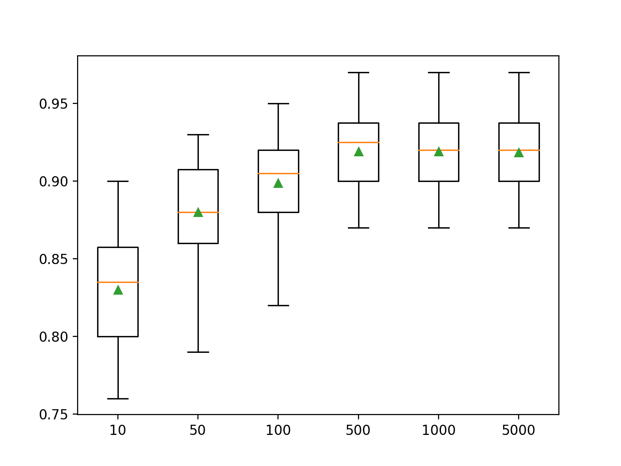
Box Plot of Gradient Boosting Ensemble Size vs. Classification Accuracy
Explore Number of Samples
The number of samples used to fit each tree can be varied. This means that each tree is fit on a randomly selected subset of the training dataset.
Using fewer samples introduces more variance for each tree, although it can improve the overall performance of the model.
The number of samples used to fit each tree is specified by the “subsample” argument and can be set to a fraction of the training dataset size. By default, it is set to 1.0 to use the entire training dataset.
The example below demonstrates the effect of the sample size on model performance.
|
1 2 3 4 5 6 7 8 9 10 11 12 13 14 15 16 17 18 19 20 21 22 23 24 25 26 27 28 29 30 31 32 33 34 35 36 37 38 39 40 41 42 43 44 45 46 47 48 49 |
# explore gradient boosting ensemble number of samples effect on performance from numpy import mean from numpy import std from numpy import arange from sklearn.datasets import make_classification from sklearn.model_selection import cross_val_score from sklearn.model_selection import RepeatedStratifiedKFold from sklearn.ensemble import GradientBoostingClassifier from matplotlib import pyplot # get the dataset def get_dataset(): X, y = make_classification(n_samples=1000, n_features=20, n_informative=15, n_redundant=5, random_state=7) return X, y # get a list of models to evaluate def get_models(): models = dict() # explore sample ratio from 10% to 100% in 10% increments for i in arange(0.1, 1.1, 0.1): key = '%.1f' % i models[key] = GradientBoostingClassifier(subsample=i) return models # evaluate a given model using cross-validation def evaluate_model(model, X, y): # define the evaluation procedure cv = RepeatedStratifiedKFold(n_splits=10, n_repeats=3, random_state=1) # evaluate the model and collect the results scores = cross_val_score(model, X, y, scoring='accuracy', cv=cv, n_jobs=-1) return scores # define dataset X, y = get_dataset() # get the models to evaluate models = get_models() # evaluate the models and store results results, names = list(), list() for name, model in models.items(): # evaluate the model scores = evaluate_model(model, X, y) # store the results results.append(scores) names.append(name) # summarize the performance along the way print('>%s %.3f (%.3f)' % (name, mean(scores), std(scores))) # plot model performance for comparison pyplot.boxplot(results, labels=names, showmeans=True) pyplot.show() |
Running the example first reports the mean accuracy for each configured sample size.
Note: Your results may vary given the stochastic nature of the algorithm or evaluation procedure, or differences in numerical precision. Consider running the example a few times and compare the average outcome.
In this case, we can see that mean performance is probably best for a sample size that is about half the size of the training dataset, such as 0.4 or higher.
|
1 2 3 4 5 6 7 8 9 10 |
>0.1 0.872 (0.033) >0.2 0.897 (0.032) >0.3 0.904 (0.029) >0.4 0.907 (0.032) >0.5 0.906 (0.027) >0.6 0.908 (0.030) >0.7 0.902 (0.032) >0.8 0.901 (0.031) >0.9 0.904 (0.031) >1.0 0.899 (0.030) |
A box and whisker plot is created for the distribution of accuracy scores for each configured number of trees.
We can see the general trend of increasing model performance perhaps peaking around 0.4 and staying somewhat level.
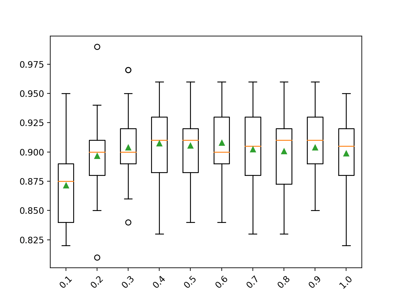
Box Plot of Gradient Boosting Ensemble Sample Size vs. Classification Accuracy
Explore Number of Features
The number of features used to fit each decision tree can be varied.
Like changing the number of samples, changing the number of features introduces additional variance into the model, which may improve performance, although it might require an increase in the number of trees.
The number of features used by each tree is taken as a random sample and is specified by the “max_features” argument and defaults to all features in the training dataset.
The example below explores the effect of the number of features on model performance for the test dataset between 1 and 20.
|
1 2 3 4 5 6 7 8 9 10 11 12 13 14 15 16 17 18 19 20 21 22 23 24 25 26 27 28 29 30 31 32 33 34 35 36 37 38 39 40 41 42 43 44 45 46 47 |
# explore gradient boosting number of features on performance from numpy import mean from numpy import std from sklearn.datasets import make_classification from sklearn.model_selection import cross_val_score from sklearn.model_selection import RepeatedStratifiedKFold from sklearn.ensemble import GradientBoostingClassifier from matplotlib import pyplot # get the dataset def get_dataset(): X, y = make_classification(n_samples=1000, n_features=20, n_informative=15, n_redundant=5, random_state=7) return X, y # get a list of models to evaluate def get_models(): models = dict() # explore number of features from 1 to 20 for i in range(1,21): models[str(i)] = GradientBoostingClassifier(max_features=i) return models # evaluate a given model using cross-validation def evaluate_model(model, X, y): # define the evaluation procedure cv = RepeatedStratifiedKFold(n_splits=10, n_repeats=3, random_state=1) # evaluate the model and collect the results scores = cross_val_score(model, X, y, scoring='accuracy', cv=cv, n_jobs=-1) return scores # define dataset X, y = get_dataset() # get the models to evaluate models = get_models() # evaluate the models and store results results, names = list(), list() for name, model in models.items(): # evaluate the model scores = evaluate_model(model, X, y) # store the results results.append(scores) names.append(name) # summarize the performance along the way print('>%s %.3f (%.3f)' % (name, mean(scores), std(scores))) # plot model performance for comparison pyplot.boxplot(results, labels=names, showmeans=True) pyplot.show() |
Running the example first reports the mean accuracy for each configured number of features.
Note: Your results may vary given the stochastic nature of the algorithm or evaluation procedure, or differences in numerical precision. Consider running the example a few times and compare the average outcome.
In this case, we can see that mean performance increases to about half the number of features and stays somewhat level after that. It’s surprising that removing half of the input variables has so little effect.
|
1 2 3 4 5 6 7 8 9 10 11 12 13 14 15 16 17 18 19 20 |
>1 0.864 (0.036) >2 0.885 (0.032) >3 0.891 (0.031) >4 0.893 (0.036) >5 0.898 (0.030) >6 0.898 (0.032) >7 0.892 (0.032) >8 0.901 (0.032) >9 0.900 (0.029) >10 0.895 (0.034) >11 0.899 (0.032) >12 0.899 (0.030) >13 0.898 (0.029) >14 0.900 (0.033) >15 0.901 (0.032) >16 0.897 (0.028) >17 0.902 (0.034) >18 0.899 (0.032) >19 0.899 (0.032) >20 0.899 (0.030) |
A box and whisker plot is created for the distribution of accuracy scores for each configured number of trees.
We can see the general trend of increasing model performance perhaps peaking around eight or nine features and staying somewhat level.
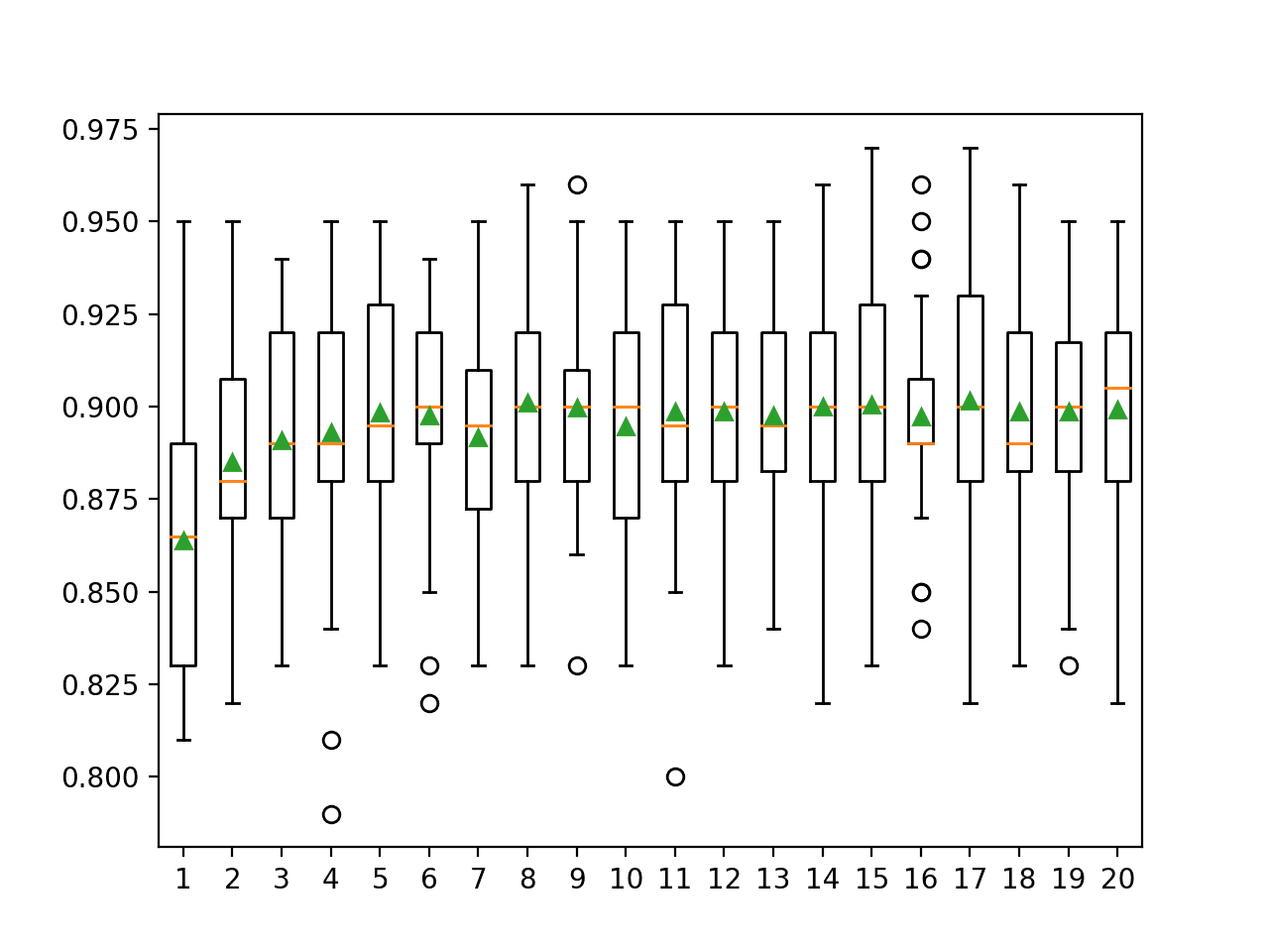
Box Plot of Gradient Boosting Ensemble Number of Features vs. Classification Accuracy
Explore Learning Rate
Learning rate controls the amount of contribution that each model has on the ensemble prediction.
Smaller rates may require more decision trees in the ensemble, whereas larger rates may require an ensemble with fewer trees. It is common to explore learning rate values on a log scale, such as between a very small value like 0.0001 and 1.0.
The learning rate can be controlled via the “learning_rate” argument and defaults to 0.1.
The example below explores the learning rate and compares the effect of values between 0.0001 and 1.0.
|
1 2 3 4 5 6 7 8 9 10 11 12 13 14 15 16 17 18 19 20 21 22 23 24 25 26 27 28 29 30 31 32 33 34 35 36 37 38 39 40 41 42 43 44 45 46 47 48 |
# explore gradient boosting ensemble learning rate effect on performance from numpy import mean from numpy import std from sklearn.datasets import make_classification from sklearn.model_selection import cross_val_score from sklearn.model_selection import RepeatedStratifiedKFold from sklearn.ensemble import GradientBoostingClassifier from matplotlib import pyplot # get the dataset def get_dataset(): X, y = make_classification(n_samples=1000, n_features=20, n_informative=15, n_redundant=5, random_state=7) return X, y # get a list of models to evaluate def get_models(): models = dict() # define learning rates to explore for i in [0.0001, 0.001, 0.01, 0.1, 1.0]: key = '%.4f' % i models[key] = GradientBoostingClassifier(learning_rate=i) return models # evaluate a given model using cross-validation def evaluate_model(model, X, y): # define the evaluation procedure cv = RepeatedStratifiedKFold(n_splits=10, n_repeats=3, random_state=1) # evaluate the model and collect the results scores = cross_val_score(model, X, y, scoring='accuracy', cv=cv, n_jobs=-1) return scores # define dataset X, y = get_dataset() # get the models to evaluate models = get_models() # evaluate the models and store results results, names = list(), list() for name, model in models.items(): # evaluate the model scores = evaluate_model(model, X, y) # store the results results.append(scores) names.append(name) # summarize the performance along the way print('>%s %.3f (%.3f)' % (name, mean(scores), std(scores))) # plot model performance for comparison pyplot.boxplot(results, labels=names, showmeans=True) pyplot.show() |
Running the example first reports the mean accuracy for each configured learning rate.
Note: Your results may vary given the stochastic nature of the algorithm or evaluation procedure, or differences in numerical precision. Consider running the example a few times and compare the average outcome.
In this case, we can see that a larger learning rate results in better performance on this dataset. We would expect that adding more trees to the ensemble for the smaller learning rates would further lift performance.
This highlights the trade-off between the number of trees (speed of training) and learning rate, e.g. we can fit a model faster by using fewer trees and a larger learning rate.
|
1 2 3 4 5 |
>0.0001 0.761 (0.043) >0.0010 0.781 (0.034) >0.0100 0.836 (0.034) >0.1000 0.899 (0.030) >1.0000 0.908 (0.025) |
A box and whisker plot is created for the distribution of accuracy scores for each configured number of trees.
We can see the general trend of increasing model performance with the increase in learning rate.
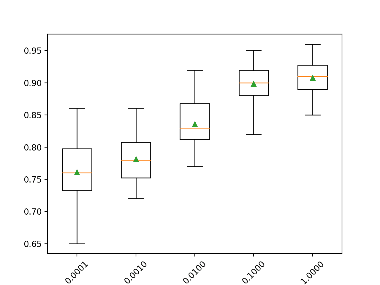
Box Plot of Gradient Boosting Ensemble Learning Rate vs. Classification Accuracy
Explore Tree Depth
Like varying the number of samples and features used to fit each decision tree, varying the depth of each tree is another important hyperparameter for gradient boosting.
The tree depth controls how specialized each tree is to the training dataset: how general or overfit it might be. Trees are preferred that are not too shallow and general (like AdaBoost) and not too deep and specialized (like bootstrap aggregation).
Gradient boosting performs well with trees that have a modest depth finding a balance between skill and generality.
Tree depth is controlled via the “max_depth” argument and defaults to 3.
The example below explores tree depths between 1 and 10 and the effect on model performance.
|
1 2 3 4 5 6 7 8 9 10 11 12 13 14 15 16 17 18 19 20 21 22 23 24 25 26 27 28 29 30 31 32 33 34 35 36 37 38 39 40 41 42 43 44 45 46 47 |
# explore gradient boosting tree depth effect on performance from numpy import mean from numpy import std from sklearn.datasets import make_classification from sklearn.model_selection import cross_val_score from sklearn.model_selection import RepeatedStratifiedKFold from sklearn.ensemble import GradientBoostingClassifier from matplotlib import pyplot # get the dataset def get_dataset(): X, y = make_classification(n_samples=1000, n_features=20, n_informative=15, n_redundant=5, random_state=7) return X, y # get a list of models to evaluate def get_models(): models = dict() # define max tree depths to explore between 1 and 10 for i in range(1,11): models[str(i)] = GradientBoostingClassifier(max_depth=i) return models # evaluate a given model using cross-validation def evaluate_model(model, X, y): # define the evaluation procedure cv = RepeatedStratifiedKFold(n_splits=10, n_repeats=3, random_state=1) # evaluate the model and collect the results scores = cross_val_score(model, X, y, scoring='accuracy', cv=cv, n_jobs=-1) return scores # define dataset X, y = get_dataset() # get the models to evaluate models = get_models() # evaluate the models and store results results, names = list(), list() for name, model in models.items(): # evaluate the model scores = evaluate_model(model, X, y) # store the results results.append(scores) names.append(name) # summarize the performance along the way print('>%s %.3f (%.3f)' % (name, mean(scores), std(scores))) # plot model performance for comparison pyplot.boxplot(results, labels=names, showmeans=True) pyplot.show() |
Running the example first reports the mean accuracy for each configured tree depth.
Note: Your results may vary given the stochastic nature of the algorithm or evaluation procedure, or differences in numerical precision. Consider running the example a few times and compare the average outcome.
In this case, we can see that performance improves with tree depth, perhaps peaking around a depth of 3 to 6, after which the deeper, more specialized trees result in worse performance.
|
1 2 3 4 5 6 7 8 9 10 |
>1 0.834 (0.031) >2 0.877 (0.029) >3 0.899 (0.030) >4 0.905 (0.032) >5 0.916 (0.030) >6 0.912 (0.031) >7 0.908 (0.033) >8 0.888 (0.031) >9 0.853 (0.036) >10 0.835 (0.034) |
A box and whisker plot is created for the distribution of accuracy scores for each configured tree depth.
We can see the general trend of increasing model performance with the tree depth to a point, after which performance begins to degrade rapidly with the over-specialized trees.
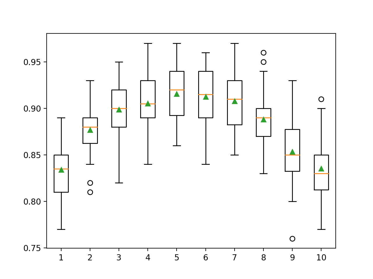
Box Plot of Gradient Boosting Ensemble Tree Depth vs. Classification Accuracy
Grid Search Hyperparameters
Gradient boosting can be challenging to configure as the algorithm as many key hyperparameters that influence the behavior of the model on training data and the hyperparameters interact with each other.
As such, it is a good practice to use a search process to discover a configuration of the model hyperparameters that works well or best for a given predictive modeling problem. Popular search processes include a random search and a grid search.
In this section we will look at grid searching common ranges for the key hyperparameters for the gradient boosting algorithm that you can use as starting point for your own projects. This can be achieving using the GridSearchCV class and specifying a dictionary that maps model hyperparameter names to the values to search.
In this case, we will grid search four key hyperparameters for gradient boosting: the number of trees used in the ensemble, the learning rate, subsample size used to train each tree, and the maximum depth of each tree. We will use a range of popular well performing values for each hyperparameter.
Each configuration combination will be evaluated using repeated k-fold cross-validation and configurations will be compared using the mean score, in this case, classification accuracy.
The complete example of grid searching the key hyperparameters of the gradient boosting algorithm on our synthetic classification dataset is listed below.
|
1 2 3 4 5 6 7 8 9 10 11 12 13 14 15 16 17 18 19 20 21 22 23 24 25 26 27 28 29 |
# example of grid searching key hyperparameters for gradient boosting on a classification dataset from sklearn.datasets import make_classification from sklearn.model_selection import RepeatedStratifiedKFold from sklearn.model_selection import GridSearchCV from sklearn.ensemble import GradientBoostingClassifier # define dataset X, y = make_classification(n_samples=1000, n_features=20, n_informative=15, n_redundant=5, random_state=7) # define the model with default hyperparameters model = GradientBoostingClassifier() # define the grid of values to search grid = dict() grid['n_estimators'] = [10, 50, 100, 500] grid['learning_rate'] = [0.0001, 0.001, 0.01, 0.1, 1.0] grid['subsample'] = [0.5, 0.7, 1.0] grid['max_depth'] = [3, 7, 9] # define the evaluation procedure cv = RepeatedStratifiedKFold(n_splits=10, n_repeats=3, random_state=1) # define the grid search procedure grid_search = GridSearchCV(estimator=model, param_grid=grid, n_jobs=-1, cv=cv, scoring='accuracy') # execute the grid search grid_result = grid_search.fit(X, y) # summarize the best score and configuration print("Best: %f using %s" % (grid_result.best_score_, grid_result.best_params_)) # summarize all scores that were evaluated means = grid_result.cv_results_['mean_test_score'] stds = grid_result.cv_results_['std_test_score'] params = grid_result.cv_results_['params'] for mean, stdev, param in zip(means, stds, params): print("%f (%f) with: %r" % (mean, stdev, param)) |
Running the example many take a while depending on your hardware. At the end of the run, the configuration that achieved the best score is reported first, followed by the scores for all other configurations that were considered.
Note: Your results may vary given the stochastic nature of the algorithm or evaluation procedure, or differences in numerical precision. Consider running the example a few times and compare the average outcome.
In this case, we can see that a configuration with a learning rate of 0.1, max depth of 7 levels, 500 trees and a subsample of 70% performed the best with a classification accuracy of about 94.6 percent.
The model may perform even better with more trees such as 1,000 or 5,000 although these configurations were not tested in this case to ensure that the grid search completed in a reasonable time.
|
1 2 3 4 5 6 7 |
Best: 0.946667 using {'learning_rate': 0.1, 'max_depth': 7, 'n_estimators': 500, 'subsample': 0.7} 0.529667 (0.089012) with: {'learning_rate': 0.0001, 'max_depth': 3, 'n_estimators': 10, 'subsample': 0.5} 0.525667 (0.077875) with: {'learning_rate': 0.0001, 'max_depth': 3, 'n_estimators': 10, 'subsample': 0.7} 0.524000 (0.072874) with: {'learning_rate': 0.0001, 'max_depth': 3, 'n_estimators': 10, 'subsample': 1.0} 0.772667 (0.037500) with: {'learning_rate': 0.0001, 'max_depth': 3, 'n_estimators': 50, 'subsample': 0.5} 0.767000 (0.037696) with: {'learning_rate': 0.0001, 'max_depth': 3, 'n_estimators': 50, 'subsample': 0.7} ... |
Common Questions
In this section we will take a closer look at some common sticking points you may have with the gradient boosting ensemble procedure.
Q. What algorithm should be used in the ensemble?
Technically any high variance algorithm that support instance weighting can be used as the basis for the ensemble.
The most common algorithm to use for speed and model performance is a decision tree with a limited tree depth, such as between 4 and 8 levels.
Q. How many ensemble members should be used?
The number of trees in the ensemble should be tuned based on the specific of the dataset and other hyperparametres such as the learning rate.
Q. Won’t the ensemble overfit with too many trees?
Yes, gradient boosting models can overfit.
It is important to carefully choose model hyperparameters using a search procedure, such as a grid search.
The learning rate, also called shrinkage, can be set to smaller values in order to slow down the rate of learning with the increase of the number of models used in the ensemble and in turn reduce the effect of overfitting.
Q. What are the downsides of gradient boosting?
Gradient boosting can be challenging to configure, often requiring a grid search or similar search procedure.
It can be very slow to train a gradient boosting model as trees must be added sequentially, unlike bagging and stacking based models where ensemble members can be trained in parallel.
Q. What problems are well suited to boosting?
Gradient boosting performs well on a wide range of regression and classification predictive modeling problems.
It might be one of the most popular algorithms for structured data (tabular data) given that it performs so well on average.
Further Reading
This section provides more resources on the topic if you are looking to go deeper.
Tutorials
- A Gentle Introduction to the Gradient Boosting Algorithm for Machine Learning
- How to Configure the Gradient Boosting Algorithm
- Gradient Boosting with Scikit-Learn, XGBoost, LightGBM, and CatBoost
Papers
- Arcing the edge, 1998.
- Stochastic Gradient Boosting, 1999.
- Boosting Algorithms as Gradient Descent in Function Space, 1999.
APIs
Articles
Summary
In this tutorial, you discovered how to develop Gradient Boosting ensembles for classification and regression.
Specifically, you learned:
- Gradient Boosting ensemble is an ensemble created from decision trees added sequentially to the model.
- How to use the Gradient Boosting ensemble for classification and regression with scikit-learn.
- How to explore the effect of Gradient Boosting model hyperparameters on model performance.
Do you have any questions?
Ask your questions in the comments below and I will do my best to answer.
Get a Handle on Modern Ensemble Learning!

Improve Your Predictions in Minutes
...with just a few lines of python code
Discover how in my new Ebook:
Ensemble Learning Algorithms With Python
It provides self-study tutorials with full working code on:
Stacking, Voting, Boosting, Bagging, Blending, Super Learner,
and much more...
 Ensemble in Python")
 Ensemble")


Dear Dr Jason,
I have a question about the GradientBoostingClassifier.
In your examples, you had y which was either 0 or 1.
My question can the GradientBoostingClassifier be used for y which consists of values of 0 or 1 or 2 or 3.
Put it another way – can GradientBoostingClassifier be used to predict values 0 or 1 or 2 or 3 integers?
Thank you,
Anthony of Sydney
Yes, this is multi-class classification and gradient boosting supports it.
Dear Dr Jason,
I have one further question.
We know that the make_classification function will generate gaussian features and integer, dependent variable y.
We also know that make_classification can also generate not only 0/1 but 0,1,2,3,4 discrete values.
First question::
I put a question to the stackexchange forum on whether there is a function that is similar to make_classification but instead of generating gaussian features, whether there is a function that generates integer features?
So far no reply from the stackexchange forum for over a week.
Second question
Suppose we can make our own version of make_classification_with_integer_features, can we use the following function:
Thank you,
Anthony of Sydney
I’m not aware of such a built in function, sorry, I don’t have the capacity to prepare such a function for you.
Dear Dr Jason,
Thank you for your reply. I was not asking anyone to make a function if the function was not available/ready-made. I could write this myself.
Suppose I wrote a generation function that generates the classification Y belonging to the set of integers and the features, X belonging to the set of integers, and call that function:
Can the cross_val_score function calculate the score for features X belonging to the set of integers?
Thank you,
Anthony of Sydney
If the target is classification, the stratified cross-validation scheme is agnostic to the data types of the inputs.
Dear Dr Jason,
Many thanks for that.
I am in the process of developing a function that accepts X belonging to the set of integers and y belonging to the set of integers. It is a prototype and when I have something that works, I will put it underneath here.
Thank you,
Anthony of Sydney
Great!
Dear Dr Jason,
Here is my implementation of make_classification_Y_with_integer_features_X
Now I will generate a set with 1000 samples and 20 features.
Appears to work, needs improvement in the model generation especially with the distribution of the features X and classification Y. For example, poisson distribution.
Question – interpretation of score 0.52
Thank you
Anthony of Sydney
Well done!
More on standard deviation here:
https://en.wikipedia.org/wiki/Standard_deviation
Thanks, helped a lot.
You’re welcome!
Thanks for making this platform, i always use it to get a hands-on on any ml algo i learn. I have a que regarding subspample parameter in gradientboosting, as when we add another tree, we try to fix the residual error, how can subsample reduce variance ?
You’re welcome.
Hmmm. Off the cuff, subsample would increase the variance, not reduce it.
If I have multiple customers with varying data sets (ie cust 1 – 36 months of data and customer 2 – 12 months of data) what is the quickest way to see if the model worked effectively on all customers if I set the model on training data at the same time for customers. I have over 600,000 customers w varying lengths of historical data……
Perhaps evaluate your model on a representative sample of customers from your larger dataset.
is there any implementation of the algorithm from scratch in numpy ? couldnt find.
I don’t know sorry. I don’t think I have one yet.
Hi Jason,
Thanks for this great tutorial
Can we use the gradient boosting algorithm for any model other than decision trees?
Do you recommend any tutorials for this?
Thanks
Yes or maybe depending on the complexity of the boosting you’re doing, although other methods do not work well.