How to Get Good Results Fast with Deep Learning for Time Series Forecasting

3 Strategies to Design Experiments and Manage Complexity on
Your Predictive Modeling Problem.

It is difficult to get started on a new time series forecasting project.

Given years of data, it can take days or weeks to fit a deep learning model. How do you get started exactly?

For some practitioners, this can lead to paralysis and even procrastination at the very beginning of a project. In others, it can result in being caught in the trap of only trying and using what has worked before rather than truly exploring the problem.

In this post, you will discover practical strategies that you can use to get started when applying deep learning methods like Multilayer Neural Networks and Long Short-Term Memory (LSTM) Recurrent Neural Network models to time series forecasting problems.

The strategies in this post are not foolproof, but they are hard learned rules of thumb that I have discovered while working with large time series datasets.

After reading this post, you will know:

• A strategy to balance the exploration of ideas and the exploitation of what works on your problem.
• A strategy to learn quickly and scale ideas with data to confirm they hold on the broader problem.
• A strategy to navigate the complexity of the framing of your problem and the complexity of the chosen deep learning model.

Kick-start your project with my new book Deep Learning for Time Series Forecasting, including step-by-step tutorials and the Python source code files for all examples.

Let’s get started.

1. Strategy for Exploration and Exploitation

It is important to balance exploration and exploitation in your search for a model that performs well on your problem.

I would recommend two different approaches that should be used in tandem:

• Diagnostics.
• Grid Search.

Diagnostics

Diagnostics involve performing a run with one set of hyperparameters and producing a trace of the model skill on the training and test dataset each training epoch.

These plots provide insight into over-learning or under-learning and the potential for specific sets of hyperparameters.

They are sanity checks or seeds for deeper investigation of ranges of parameters that can be explored and prevent you from wasting time with more epochs than are reasonably required, or networks that are too large.

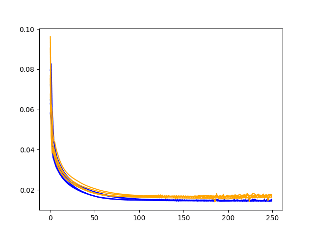
Below is an example of a diagnostic plot from a model run showing training and validation RMSE.

Example Diagnostic Line Plot Comparing Train and Test Loss Over Training Epochs

Grid Search

Based on learnings from diagnostic results, the grid search provides a sweep across a suite of values for specific model hyperparameters such as the number of neurons, batch size, and so on.

They allow you to systematically dial in specific hyperparameter values in a piecewise manner.

Interleave the Approaches

I would recommend interleaving diagnostic runs and grid search runs.

You can spot check your hypotheses with diagnostics and get the best from promising ideas with grid search results.

I would strongly encourage you to test every assumption you have about the model. This includes simple things like data scaling, weight initialization, and even the choice of activation function, loss function, and more.

Used with the data handling strategy below, you will quickly build a map of what works and what doesn’t on your forecasting problem.

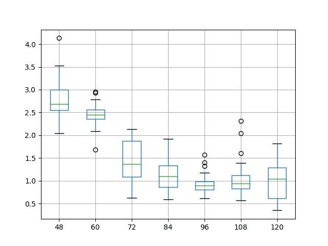
Below is an example of the results of a grid search of the batch size for a model showing the distribution of the results of each experiment repeated 30 times.

Example Box and Whisker Plots Comparing a Model Skill For Different Model Parameter Values

2. Strategy for Handling Data Size

I recommend a strategy of working with smaller samples of data first to test ideas and slowly increasing the amount of data to see if things learned on the small samples hold on larger samples.

For example, if you have multiple years of hourly measurements, you could split your data as follows:

• 1 week sample.
• 1 month sample.
• 1 year sample.
• all data.

The alternative is that you fit and explore models on the entire dataset where each model can take days to fit, in turn meaning that your rate of learning is dramatically decreased.

The benefit of this approach is that you can very quickly test ideas, in minutes, with multiple repeats (e.g. statistically significant) and then later scale up only those promising ideas to more and more data.

Generally, with well-framed supervised learning problems, the learnings do scale with the data. Nevertheless, there is a risk that the problems are substantially different at different scales of data and that findings do not hold. You can check for this with simpler models that are faster to train and tease out whether this is an issue early on.

Finally, as you scale models to more data, you can also reduce the number of repeats of experiments to aid in speeding up the turnaround of results.

3. Strategy for Model Complexity

Like data size, the complexity of the model is another concern that must be managed and can be scaled.

We can look at this both from the framing of the supervised learning problem and the model itself.

Model Framing Complexity

For example, we may assume a time series forecasting problem that includes exogenous variables (e.g. multiple input series or multivariate inputs).

We can scale the complexity of the problem and see what works at one level of complexity (e.g. univariate inputs) holds at more complex levels of complexity (multivariate inputs).

For example, you could work through model complexity as follows:

• Univariate input, single-step output.
• Univariate input, multi-step output.
• Multivariate inputs, single-step output.
• Multivariate inputs, multi-step output.

This too can extend to multivariate forecasts.

At each step, the objective is to demonstrate that the addition of complexity can lift the skill of the model.

For example:

• Can a neural network model outperform a persistence forecast model?
• Can a neural network model outperform a linear forecast model?
• Can exogenous input variables lift the skill of the model over a univariate input?
• Can a direct a multi-step forecast be more skillful than a recursive single-step forecast?

If these questions can’t be overcome, or be overcome easily, it can help you quickly settle on a framing of the problem and a chosen type of model.

Complexity in Model Capability

This same approach can be used when working with more sophisticated neural network models like LSTMs.

For example:

• Model the problem as a mapping of inputs to outputs (e.g. no internal state or BPTT).
• Model the problem as a mapping problem with internal state across input sequences only (no BPTT).
• Model the problem as a mapping problem with internal state and BPTT.

At each step, the increased model complexity must demonstrate skill at or above the prior level of complexity. Said another way, the added model complexity must be justified by a commensurate increase in model skill or capability.

For example:

• Can an LSTM outperform an MLP with a window?
• Can an LSTM with internal state and no BPTT outperform an LSTM where the state is reset after each sample?
• Can an LSTM with BPTT over input sequences outperform an LSTM that is updated after each time step?

Further Reading

This section provides more resources on the topic if you are looking go deeper.

• How to Work Through a Time Series Forecast Project
• How to Tune LSTM Hyperparameters with Keras for Time Series Forecasting
• How To Improve Deep Learning Performance

Summary

In this tutorial, you discovered how you can overcome the paralysis that can strike at the beginning of a deep learning project.

Specifically, you learned how you can systematically break down complexity and strategies that you can use to get results fast:

• A strategy to balance the exploration of ideas and the exploitation of what works on your problem.
• A strategy to learn quickly and scale ideas with data to confirm they hold on the broader problem.
• A strategy to navigate the complexity of the framing of your problem and the complexity of your chosen deep learning model.

Do you have any questions?
Ask your questions in the comments below and I will do my best to answer.

Develop Deep Learning models for Time Series Today!

Develop Your Own Forecasting models in Minutes

...with just a few lines of python code

Discover how in my new Ebook:
Deep Learning for Time Series Forecasting

It provides self-study tutorials on topics like:
CNNs, LSTMs, Multivariate Forecasting, Multi-Step Forecasting and much more...

Finally Bring Deep Learning to your Time Series Forecasting Projects

Skip the Academics. Just Results.

See What's Inside