
Caption generation is a challenging artificial intelligence problem where a textual description must be generated for a photograph.
It requires both methods from computer vision to understand the content of the image and a language model from the field of natural language processing to turn the understanding of the image into words in the right order. Recently, deep learning methods have achieved state of the art results on examples of this problem.
It can be hard to develop caption generating models on your own data, primarily because the datasets and the models are so large and take days to train. An alternative approach is to explore model configurations with a small sample of the fuller dataset.
In this tutorial, you will discover how you can use a small sample of a standard photo captioning dataset to explore different deep model designs.
After completing this tutorial, you will know:
- How to prepare data for photo captioning modeling.
- How to design a baseline and test harness to evaluate the skill of models and control for their stochastic nature.
- How to evaluate properties like model skill, feature extraction models, and word embeddings in order to lift model skill.
Kick-start your project with my new book Deep Learning for Natural Language Processing, including step-by-step tutorials and the Python source code files for all examples.
Let’s get started.
- April Feb/2019: Provided direct links for the Flickr8k_Dataset dataset, as the official site was taken down.
How to Use Small Experiments to Develop a Caption Generation Model in Keras
Photo by Per, some rights reserved.
Tutorial Overview
This tutorial is divided into 6 parts; they are:
- Data Preparation
- Baseline Caption Generation Model
- Network Size Parameters
- Configuring the Feature Extraction Model
- Word Embedding Models
- Analysis of Results
Python Environment
This tutorial assumes you have a Python SciPy environment installed, ideally with Python 3.
You must have Keras (2.0 or higher) installed with either the TensorFlow or Theano backend.
The tutorial also assumes you have scikit-learn, Pandas, NumPy, and Matplotlib installed.
If you need help with your environment, see this tutorial:
I recommend running the code on a system with a GPU.
You can access GPUs cheaply on Amazon Web Services. Learn how in this tutorial:
Let’s dive in.
Need help with Deep Learning for Text Data?
Take my free 7-day email crash course now (with code).
Click to sign-up and also get a free PDF Ebook version of the course.
Data Preparation
First, we need to prepare the dataset for training the model.
We will use the Flickr8K dataset that is comprised of a little more than 8,000 photographs and their descriptions.
You can download the dataset from here:
UPDATE (April/2019): The official site seems to have been taken down (although the form still works). Here are some direct download links from my datasets GitHub repository:
Unzip the photographs and descriptions into your current working directory into Flicker8k_Dataset and Flickr8k_text directories respectively.
There are two parts to the data preparation, they are:
- Preparing the Text
- Preparing the Photos
Preparing the Text
The dataset contains multiple descriptions for each photograph and the text of the descriptions requires some minimal cleaning.
First, we will load the file containing all of the descriptions.
|
1 2 3 4 5 6 7 8 9 10 11 12 13 |
# load doc into memory def load_doc(filename): # open the file as read only file = open(filename, 'r') # read all text text = file.read() # close the file file.close() return text filename = 'Flickr8k_text/Flickr8k.token.txt' # load descriptions doc = load_doc(filename) |
Each photo has a unique identifier. This is used in the photo filename and in the text file of descriptions. Next, we will step through the list of photo descriptions and save the first description for each photo. Below defines a function named load_descriptions() that, given the loaded document text, will return a dictionary of photo identifiers to descriptions.
|
1 2 3 4 5 6 7 8 9 10 11 12 13 14 15 16 17 18 19 20 21 22 23 |
# extract descriptions for images def load_descriptions(doc): mapping = dict() # process lines for line in doc.split('\n'): # split line by white space tokens = line.split() if len(line) < 2: continue # take the first token as the image id, the rest as the description image_id, image_desc = tokens[0], tokens[1:] # remove filename from image id image_id = image_id.split('.')[0] # convert description tokens back to string image_desc = ' '.join(image_desc) # store the first description for each image if image_id not in mapping: mapping[image_id] = image_desc return mapping # parse descriptions descriptions = load_descriptions(doc) print('Loaded: %d ' % len(descriptions)) |
Next, we need to clean the description text.
The descriptions are already tokenized and easy to work with. We will clean the text in the following ways in order to reduce the size of the vocabulary of words we will need to work with:
- Convert all words to lowercase.
- Remove all punctuation.
- Remove all words that are one character or less in length (e.g. ‘a’).
Below defines the clean_descriptions() function that, given the dictionary of image identifiers to descriptions, steps through each description and cleans the text.
|
1 2 3 4 5 6 7 8 9 10 11 12 13 14 15 16 17 18 19 20 21 22 23 |
import string def clean_descriptions(descriptions): # prepare translation table for removing punctuation table = str.maketrans('', '', string.punctuation) for key, desc in descriptions.items(): # tokenize desc = desc.split() # convert to lower case desc = [word.lower() for word in desc] # remove punctuation from each token desc = [w.translate(table) for w in desc] # remove hanging 's' and 'a' desc = [word for word in desc if len(word)>1] # store as string descriptions[key] = ' '.join(desc) # clean descriptions clean_descriptions(descriptions) # summarize vocabulary all_tokens = ' '.join(descriptions.values()).split() vocabulary = set(all_tokens) print('Vocabulary Size: %d' % len(vocabulary)) |
Finally, we save the dictionary of image identifiers and descriptions to a new file named descriptions.txt, with one image identifier and description per line.
Below defines the save_doc() function that given a dictionary containing the mapping of identifiers to descriptions and a filename, saves the mapping to file.
|
1 2 3 4 5 6 7 8 9 10 11 12 |
# save descriptions to file, one per line def save_doc(descriptions, filename): lines = list() for key, desc in descriptions.items(): lines.append(key + ' ' + desc) data = '\n'.join(lines) file = open(filename, 'w') file.write(data) file.close() # save descriptions save_doc(descriptions, 'descriptions.txt') |
Putting this all together, the complete listing is provided below.
|
1 2 3 4 5 6 7 8 9 10 11 12 13 14 15 16 17 18 19 20 21 22 23 24 25 26 27 28 29 30 31 32 33 34 35 36 37 38 39 40 41 42 43 44 45 46 47 48 49 50 51 52 53 54 55 56 57 58 59 60 61 62 63 64 65 66 67 68 69 70 71 |
import string # load doc into memory def load_doc(filename): # open the file as read only file = open(filename, 'r') # read all text text = file.read() # close the file file.close() return text # extract descriptions for images def load_descriptions(doc): mapping = dict() # process lines for line in doc.split('\n'): # split line by white space tokens = line.split() if len(line) < 2: continue # take the first token as the image id, the rest as the description image_id, image_desc = tokens[0], tokens[1:] # remove filename from image id image_id = image_id.split('.')[0] # convert description tokens back to string image_desc = ' '.join(image_desc) # store the first description for each image if image_id not in mapping: mapping[image_id] = image_desc return mapping def clean_descriptions(descriptions): # prepare translation table for removing punctuation table = str.maketrans('', '', string.punctuation) for key, desc in descriptions.items(): # tokenize desc = desc.split() # convert to lower case desc = [word.lower() for word in desc] # remove punctuation from each token desc = [w.translate(table) for w in desc] # remove hanging 's' and 'a' desc = [word for word in desc if len(word)>1] # store as string descriptions[key] = ' '.join(desc) # save descriptions to file, one per line def save_doc(descriptions, filename): lines = list() for key, desc in descriptions.items(): lines.append(key + ' ' + desc) data = '\n'.join(lines) file = open(filename, 'w') file.write(data) file.close() filename = 'Flickr8k_text/Flickr8k.token.txt' # load descriptions doc = load_doc(filename) # parse descriptions descriptions = load_descriptions(doc) print('Loaded: %d ' % len(descriptions)) # clean descriptions clean_descriptions(descriptions) # summarize vocabulary all_tokens = ' '.join(descriptions.values()).split() vocabulary = set(all_tokens) print('Vocabulary Size: %d' % len(vocabulary)) # save descriptions save_doc(descriptions, 'descriptions.txt') |
Running the example first prints the number of loaded photo descriptions (8,092) and the size of the clean vocabulary (4,484 words).
|
1 2 |
Loaded: 8092 Vocabulary Size: 4484 |
The clean descriptions are then written to ‘descriptions.txt‘. Taking a look in the file, we can see that the descriptions are ready for modeling.
Taking a look in the file, we can see that the descriptions are ready for modeling.
|
1 2 3 4 5 6 |
3621647714_fc67ab2617 man is standing on snow with trees and mountains all around him 365128300_6966058139 group of people are rafting on river rapids 2751694538_fffa3d307d man and boy sit in the driver seat 537628742_146f2c24f8 little girl running in field 2320125735_27fe729948 black and brown dog with blue collar goes on alert by soccer ball in the grass ... |
Preparing the Photos
We will use a pre-trained model to interpret the content of the photos.
There are many models to choose from. In this case, we will use the Oxford Visual Geometry Group or VGG model that won the ImageNet competition in 2014. Learn more about the model here:
Keras provides this pre-trained model directly. Note, the first time you use this model, Keras will download the model weights from the Internet, which are about 500 Megabytes. This may take a few minutes depending on your internet connection.
We could use this model as part of a broader image caption model. The problem is, it is a large model and running each photo through the network every time we want to test a new language model configuration (downstream) is redundant.
Instead, we can pre-compute the “photo features” using the pre-trained model and save them to file. We can then load these features later and feed them into our model as the interpretation of a given photo in the dataset. It is no different to running the photo through the full VGG model, it is just that we will have done it once in advance.
This is an optimization that will make training our models faster and consume less memory.
We can load the VGG model in Keras using the VGG class. We will load the model without the top; this means without the layers at the end of the network that are used to interpret the features extracted from the input and turn them into a class prediction. We are not interested in the image net classification of the photos and we will train our own interpretation of the image features.
Keras also provides tools for reshaping the loaded photo into the preferred size for the model (e.g. 3 channel 224 x 224 pixel image).
Below is a function named extract_features() that given a directory name will load each photo, prepare it for VGG and collect the predicted features from the VGG model. The image features are a 3-dimensional array with the shape (7, 7, 512).
The function returns a dictionary of image identifier to image features.
|
1 2 3 4 5 6 7 8 9 10 11 12 13 14 15 16 17 18 19 20 21 22 23 24 25 26 |
# extract features from each photo in the directory def extract_features(directory): # load the model in_layer = Input(shape=(224, 224, 3)) model = VGG16(include_top=False, input_tensor=in_layer) print(model.summary()) # extract features from each photo features = dict() for name in listdir(directory): # load an image from file filename = directory + '/' + name image = load_img(filename, target_size=(224, 224)) # convert the image pixels to a numpy array image = img_to_array(image) # reshape data for the model image = image.reshape((1, image.shape[0], image.shape[1], image.shape[2])) # prepare the image for the VGG model image = preprocess_input(image) # get features feature = model.predict(image, verbose=0) # get image id image_id = name.split('.')[0] # store feature features[image_id] = feature print('>%s' % name) return features |
We can call this function to prepare the photo data for testing our models, then save the resulting dictionary to a file named ‘features.pkl‘.
The complete example is listed below.
|
1 2 3 4 5 6 7 8 9 10 11 12 13 14 15 16 17 18 19 20 21 22 23 24 25 26 27 28 29 30 31 32 33 34 35 36 37 38 39 40 41 |
from os import listdir from pickle import dump from keras.applications.vgg16 import VGG16 from keras.preprocessing.image import load_img from keras.preprocessing.image import img_to_array from keras.applications.vgg16 import preprocess_input from keras.layers import Input # extract features from each photo in the directory def extract_features(directory): # load the model in_layer = Input(shape=(224, 224, 3)) model = VGG16(include_top=False, input_tensor=in_layer) print(model.summary()) # extract features from each photo features = dict() for name in listdir(directory): # load an image from file filename = directory + '/' + name image = load_img(filename, target_size=(224, 224)) # convert the image pixels to a numpy array image = img_to_array(image) # reshape data for the model image = image.reshape((1, image.shape[0], image.shape[1], image.shape[2])) # prepare the image for the VGG model image = preprocess_input(image) # get features feature = model.predict(image, verbose=0) # get image id image_id = name.split('.')[0] # store feature features[image_id] = feature print('>%s' % name) return features # extract features from all images directory = 'Flicker8k_Dataset' features = extract_features(directory) print('Extracted Features: %d' % len(features)) # save to file dump(features, open('features.pkl', 'wb')) |
Running this data preparation step may take a while depending on your hardware, perhaps one hour on the CPU with a modern workstation.
At the end of the run, you will have the extracted features stored in ‘features.pkl‘ for later use.
Baseline Caption Generation Model
In this section, we will define a baseline model for generating captions for photos and how to evaluate it so that it can be compared to variations on this baseline.
This section is divided into 5 parts:
- Load Data.
- Fit Model.
- Evaluate Model.
- Complete Example
- “A” versus “A” Test
- Generate Photo Captions
1. Load Data
We are not going to fit the model on all of the caption data, or even on a large sample of the data.
In this tutorial, we are interested in quickly testing a suite of different configurations of a caption model to see what works on this data. That means we need the evaluation of one model configuration to happen quickly. Toward this end, we will train the models on 100 photographs and captions, then evaluate them on both the training dataset and on a new test set of 100 photographs and captions.
First, we need to load a pre-defined subset of photographs. The provided dataset has separate sets for train, test, and development, which are really just different groups of photo identifiers. We will load the development set and use the first 100 identifiers for train and the second 100 (e.g. from 100 to 200) as the test set.
The function load_set() below will load a pre-defined set of identifiers, and we will call it with the ‘Flickr_8k.devImages.txt‘ filename as an argument.
|
1 2 3 4 5 6 7 8 9 10 11 12 13 |
# load a pre-defined list of photo identifiers def load_set(filename): doc = load_doc(filename) dataset = list() # process line by line for line in doc.split('\n'): # skip empty lines if len(line) < 1: continue # get the image identifier identifier = line.split('.')[0] dataset.append(identifier) return set(dataset) |
Next, we need to split the set into train and test sets.
We will start by ordering the identifiers by sorting them to ensure we always split them consistently across machines and runs, then take the first 100 for train and the next 100 for test.
The train_test_split() function below will create this split given the loaded set of identifiers as input.
|
1 2 3 4 5 6 |
# split a dataset into train/test elements def train_test_split(dataset): # order keys so the split is consistent ordered = sorted(dataset) # return split dataset as two new sets return set(ordered[:100]), set(ordered[100:200]) |
Now, we can load the photo descriptions using the pre-defined set of train or test identifiers.
Below is the function load_clean_descriptions() that loads the cleaned text descriptions from ‘descriptions.txt‘ for a given set of identifiers and returns a dictionary of identifier to text.
The model we will develop will generate a caption given a photo, and the caption will be generated one word at a time. The sequence of previously generated words will be provided as input. Therefore, we will need a “first word” to kick-off the generation process and a ‘last word‘ to signal the end of the caption. We will use the strings ‘startseq‘ and ‘endseq‘ for this purpose.
|
1 2 3 4 5 6 7 8 9 10 11 12 13 14 15 |
# load clean descriptions into memory def load_clean_descriptions(filename, dataset): # load document doc = load_doc(filename) descriptions = dict() for line in doc.split('\n'): # split line by white space tokens = line.split() # split id from description image_id, image_desc = tokens[0], tokens[1:] # skip images not in the set if image_id in dataset: # store descriptions[image_id] = 'startseq ' + ' '.join(image_desc) + ' endseq' return descriptions |
Next, we can load the photo features for a given dataset.
Below defines a function named load_photo_features() that loads the entire set of photo descriptions, then returns the subset of interest for a given set of photo identifiers. This is not very efficient as the loaded dictionary of all photo features is about 700 Megabytes. Nevertheless, this will get us up and running quickly.
Note, if you have a better approach, share it in the comments below.
|
1 2 3 4 5 6 7 |
# load photo features def load_photo_features(filename, dataset): # load all features all_features = load(open(filename, 'rb')) # filter features features = {k: all_features[k] for k in dataset} return features |
We can pause here and test everything developed so far.
The complete code example is listed below.
|
1 2 3 4 5 6 7 8 9 10 11 12 13 14 15 16 17 18 19 20 21 22 23 24 25 26 27 28 29 30 31 32 33 34 35 36 37 38 39 40 41 42 43 44 45 46 47 48 49 50 51 52 53 54 55 56 57 58 59 60 61 62 63 64 65 66 67 68 69 70 71 72 |
from pickle import load # load doc into memory def load_doc(filename): # open the file as read only file = open(filename, 'r') # read all text text = file.read() # close the file file.close() return text # load a pre-defined list of photo identifiers def load_set(filename): doc = load_doc(filename) dataset = list() # process line by line for line in doc.split('\n'): # skip empty lines if len(line) < 1: continue # get the image identifier identifier = line.split('.')[0] dataset.append(identifier) return set(dataset) # split a dataset into train/test elements def train_test_split(dataset): # order keys so the split is consistent ordered = sorted(dataset) # return split dataset as two new sets return set(ordered[:100]), set(ordered[100:200]) # load clean descriptions into memory def load_clean_descriptions(filename, dataset): # load document doc = load_doc(filename) descriptions = dict() for line in doc.split('\n'): # split line by white space tokens = line.split() # split id from description image_id, image_desc = tokens[0], tokens[1:] # skip images not in the set if image_id in dataset: # store descriptions[image_id] = 'startseq ' + ' '.join(image_desc) + ' endseq' return descriptions # load photo features def load_photo_features(filename, dataset): # load all features all_features = load(open(filename, 'rb')) # filter features features = {k: all_features[k] for k in dataset} return features # load dev set filename = 'Flickr8k_text/Flickr_8k.devImages.txt' dataset = load_set(filename) print('Dataset: %d' % len(dataset)) # train-test split train, test = train_test_split(dataset) print('Train=%d, Test=%d' % (len(train), len(test))) # descriptions train_descriptions = load_clean_descriptions('descriptions.txt', train) test_descriptions = load_clean_descriptions('descriptions.txt', test) print('Descriptions: train=%d, test=%d' % (len(train_descriptions), len(test_descriptions))) # photo features train_features = load_photo_features('features.pkl', train) test_features = load_photo_features('features.pkl', test) print('Photos: train=%d, test=%d' % (len(train_features), len(test_features))) |
Running this example first loads the 1,000 photo identifiers in the development dataset. A train and test set is selected and used to filter the set of clean photo descriptions and prepared image features.
We are nearly there.
|
1 2 3 4 |
Dataset: 1,000 Train=100, Test=100 Descriptions: train=100, test=100 Photos: train=100, test=100 |
The description text will need to be encoded to numbers before it can be presented to the model as in input or compared to the model’s predictions.
The first step in encoding the data is to create a consistent mapping from words to unique integer values. Keras provides the Tokenizer class that can learn this mapping from the loaded description data.
Below defines the create_tokenizer() that will fit a Tokenizer given the loaded photo description text.
|
1 2 3 4 5 6 7 8 9 10 11 |
# fit a tokenizer given caption descriptions def create_tokenizer(descriptions): lines = list(descriptions.values()) tokenizer = Tokenizer() tokenizer.fit_on_texts(lines) return tokenizer # prepare tokenizer tokenizer = create_tokenizer(descriptions) vocab_size = len(tokenizer.word_index) + 1 print('Vocabulary Size: %d' % vocab_size) |
We can now encode the text.
Each description will be split into words. The model will be provided one word and the photo and generate the next word. Then the first two words of the description will be provided to the model as input with the image to generate the next word. This is how the model will be trained.
For example, the input sequence “little girl running in field” would be split into 6 input-output pairs to train the model:
|
1 2 3 4 5 6 7 |
X1, X2 (text sequence), y (word) photo startseq, little photo startseq, little, girl photo startseq, little, girl, running photo startseq, little, girl, running, in photo startseq, little, girl, running, in, field photo startseq, little, girl, running, in, field, endseq |
Later when the model is used to generate descriptions, the generated words will be concatenated and recursively provided as input to generate a caption for an image.
The function below named create_sequences() given the tokenizer, a single clean description, the features for a photo, and the maximum description length will prepare a set of input-output pairs for training a model. Calling this function will return X1 and X2 for the arrays of image data and input sequence data and the y value for the output word.
The input sequences are integer encoded and the output word is one-hot encoded to represent the probability distribution of the expected word across the whole vocabulary of possible words.
|
1 2 3 4 5 6 7 8 9 10 11 12 13 14 15 16 17 18 19 20 |
# create sequences of images, input sequences and output words for an image def create_sequences(tokenizer, desc, image, max_length): Ximages, XSeq, y = list(), list(),list() vocab_size = len(tokenizer.word_index) + 1 # integer encode the description seq = tokenizer.texts_to_sequences([desc])[0] # split one sequence into multiple X,y pairs for i in range(1, len(seq)): # select in_seq, out_seq = seq[:i], seq[i] # pad input sequence in_seq = pad_sequences([in_seq], maxlen=max_length)[0] # encode output sequence out_seq = to_categorical([out_seq], num_classes=vocab_size)[0] # store Ximages.append(image) XSeq.append(in_seq) y.append(out_seq) # Ximages, XSeq, y = array(Ximages), array(XSeq), array(y) return [Ximages, XSeq, y] |
2. Fit Model
We are nearly ready to fit the model.
Parts of the model have already been discussed, but let’s re-iterate.
The model is based on the example laid out in the paper “Show and Tell: A Neural Image Caption Generator“, 2015.
The model involves three parts:
- Photo Feature Extractor. This is a 16-layer VGG model pre-trained on the ImageNet dataset. We have pre-processed the photos with a the VGG model (without the top) and will use the extracted features predicted by this model as input.
- Sequence Processor. This is a word embedding layer for handling the text input, followed by an LSTM layer. The LSTM output is interpreted by a Dense layer one output at a time.
- Interpreter (for lack of a better name). Both the feature extractor and sequence processor output a fixed-length vector that is the length of a maximum sequence. These are concatenated together and processed by an LSTM and Dense layer before a final prediction is made.
A conservative number of neurons is used in the base model. Specifically, a 128 Dense layer after the feature extractor, a 50-dimensionality word embedding followed by a 256 unit LSTM and 128 neuron Dense after the sequence processor, and finally a 500 unit LSTM followed by a 500 neuron Dense at the end of the network.
The model predicts a probability distribution across the vocabulary, therefore a softmax activation function is used and a categorical cross entropy loss function is minimized while fitting the network.
The function define_model() defines the baseline model, given the size of the vocabulary and the maximum length of photo descriptions. The Keras functional API is used to define the model as it provides the flexibility needed to define a model that takes two input streams and combines them.
|
1 2 3 4 5 6 7 8 9 10 11 12 13 14 15 16 17 18 19 20 21 22 23 24 |
# define the captioning model def define_model(vocab_size, max_length): # feature extractor (encoder) inputs1 = Input(shape=(7, 7, 512)) fe1 = GlobalMaxPooling2D()(inputs1) fe2 = Dense(128, activation='relu')(fe1) fe3 = RepeatVector(max_length)(fe2) # embedding inputs2 = Input(shape=(max_length,)) emb2 = Embedding(vocab_size, 50, mask_zero=True)(inputs2) emb3 = LSTM(256, return_sequences=True)(emb2) emb4 = TimeDistributed(Dense(128, activation='relu'))(emb3) # merge inputs merged = concatenate([fe3, emb4]) # language model (decoder) lm2 = LSTM(500)(merged) lm3 = Dense(500, activation='relu')(lm2) outputs = Dense(vocab_size, activation='softmax')(lm3) # tie it together [image, seq] [word] model = Model(inputs=[inputs1, inputs2], outputs=outputs) model.compile(loss='categorical_crossentropy', optimizer='adam', metrics=['accuracy']) print(model.summary()) plot_model(model, show_shapes=True, to_file='plot.png') return model |
To get a sense for the structure of the model, specifically the shapes of the layers, see the summary listed below.
|
1 2 3 4 5 6 7 8 9 10 11 12 13 14 15 16 17 18 19 20 21 22 23 24 25 26 27 28 29 30 31 32 |
____________________________________________________________________________________________________ Layer (type) Output Shape Param # Connected to ==================================================================================================== input_1 (InputLayer) (None, 7, 7, 512) 0 ____________________________________________________________________________________________________ input_2 (InputLayer) (None, 25) 0 ____________________________________________________________________________________________________ global_max_pooling2d_1 (GlobalMa (None, 512) 0 input_1[0][0] ____________________________________________________________________________________________________ embedding_1 (Embedding) (None, 25, 50) 18300 input_2[0][0] ____________________________________________________________________________________________________ dense_1 (Dense) (None, 128) 65664 global_max_pooling2d_1[0][0] ____________________________________________________________________________________________________ lstm_1 (LSTM) (None, 25, 256) 314368 embedding_1[0][0] ____________________________________________________________________________________________________ repeat_vector_1 (RepeatVector) (None, 25, 128) 0 dense_1[0][0] ____________________________________________________________________________________________________ time_distributed_1 (TimeDistribu (None, 25, 128) 32896 lstm_1[0][0] ____________________________________________________________________________________________________ concatenate_1 (Concatenate) (None, 25, 256) 0 repeat_vector_1[0][0] time_distributed_1[0][0] ____________________________________________________________________________________________________ lstm_2 (LSTM) (None, 500) 1514000 concatenate_1[0][0] ____________________________________________________________________________________________________ dense_3 (Dense) (None, 500) 250500 lstm_2[0][0] ____________________________________________________________________________________________________ dense_4 (Dense) (None, 366) 183366 dense_3[0][0] ==================================================================================================== Total params: 2,379,094 Trainable params: 2,379,094 Non-trainable params: 0 ____________________________________________________________________________________________________ |
We also create a plot to visualize the structure of the network that better helps understand the two streams of input.
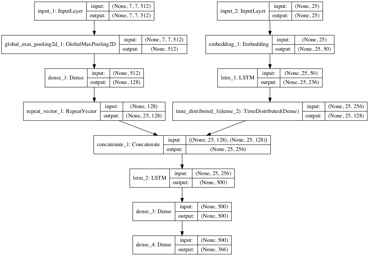
Plot of the Baseline Captioning Deep Learning Model
We will train the model using a data generator. This is strictly not required given that the captions and extracted photo features can probably fit into memory as a single dataset. Nevertheless, it is good practice for when you come to train the final model on the entire dataset.
A generator will yield a result when called. In Keras, it will yield a single batch of input-output samples that are used to estimate the error gradient and update the model weights.
The function data_generator() defines the data generator, given a dictionary of loaded photo descriptions, photo features, the tokenizer for integer encoding sequences, and the maximum sequence length in the dataset.
The generator loops forever and keeps yielding batches of input-output pairs when asked. We also have a n_step parameter that allows us to tune how many images worth of input-output pairs to generate for each batch. The average sequence has 10 words, that is 10 input-output pairs, and a good batch size might be 30 samples, which is about 2-to-3 images worth.
|
1 2 3 4 5 6 7 8 9 10 11 12 13 14 15 16 17 18 19 20 21 22 |
# data generator, intended to be used in a call to model.fit_generator() def data_generator(descriptions, features, tokenizer, max_length, n_step): # loop until we finish training while 1: # loop over photo identifiers in the dataset keys = list(descriptions.keys()) for i in range(0, len(keys), n_step): Ximages, XSeq, y = list(), list(),list() for j in range(i, min(len(keys), i+n_step)): image_id = keys[j] # retrieve photo feature input image = features[image_id][0] # retrieve text input desc = descriptions[image_id] # generate input-output pairs in_img, in_seq, out_word = create_sequences(tokenizer, desc, image, max_length) for k in range(len(in_img)): Ximages.append(in_img[k]) XSeq.append(in_seq[k]) y.append(out_word[k]) # yield this batch of samples to the model yield [[array(Ximages), array(XSeq)], array(y)] |
The model can be fit by calling fit_generator() and passing it to the data generator, along with all of the parameters needed. When fitting the model, we can also specify the number of batches to run per epoch and the number of epochs.
|
1 |
model.fit_generator(data_generator(train_descriptions, train_features, tokenizer, max_length, n_photos_per_update), steps_per_epoch=n_batches_per_epoch, epochs=n_epochs, verbose=verbose) |
For these experiments, we will use 2 images per batch, 50 batches (or 100 images) per epoch, and 50 training epochs. You can experiment with different configurations in your own experiments.
3. Evaluate Model
Now that we know how to prepare the data and define a model, we must define a test harness to evaluate a given model.
We will evaluate a model by training it on the dataset, generating descriptions for all photos in the training dataset, evaluating those predictions with a cost function, and then repeating this evaluation process multiple times.
The outcome will be a distribution of skill scores for the model that we can summarize by calculating the mean and standard deviation. This is the preferred way to evaluate deep learning models. See this post:
First, we need to be able to generate a description for a photo using a trained model.
This involves passing in the start description token ‘startseq‘, generating one word, then calling the model recursively with generated words as input until the end of sequence token is reached ‘endseq‘ or the maximum description length is reached.
The function below named generate_desc() implements this behavior and generates a textual description given a trained model, and a given prepared photo as input. It calls the function word_for_id() in order to map an integer prediction back to a word.
|
1 2 3 4 5 6 7 8 9 10 11 12 13 14 15 16 17 18 19 20 21 22 23 24 25 26 27 28 29 30 31 32 |
# map an integer to a word def word_for_id(integer, tokenizer): for word, index in tokenizer.word_index.items(): if index == integer: return word return None # generate a description for an image def generate_desc(model, tokenizer, photo, max_length): # seed the generation process in_text = 'startseq' # iterate over the whole length of the sequence for i in range(max_length): # integer encode input sequence sequence = tokenizer.texts_to_sequences([in_text])[0] # pad input sequence = pad_sequences([sequence], maxlen=max_length) # predict next word yhat = model.predict([photo,sequence], verbose=0) # convert probability to integer yhat = argmax(yhat) # map integer to word word = word_for_id(yhat, tokenizer) # stop if we cannot map the word if word is None: break # append as input for generating the next word in_text += ' ' + word # stop if we predict the end of the sequence if word == 'endseq': break return in_text |
We will generate predictions for all photos in the training dataset and in the test dataset.
The function below named evaluate_model() will evaluate a trained model against a given dataset of photo descriptions and photo features. The actual and predicted descriptions are collected and evaluated collectively using the corpus BLEU score that summarizes how close the generated text is to the expected text.
|
1 2 3 4 5 6 7 8 9 10 11 12 13 |
# evaluate the skill of the model def evaluate_model(model, descriptions, photos, tokenizer, max_length): actual, predicted = list(), list() # step over the whole set for key, desc in descriptions.items(): # generate description yhat = generate_desc(model, tokenizer, photos[key], max_length) # store actual and predicted actual.append([desc.split()]) predicted.append(yhat.split()) # calculate BLEU score bleu = corpus_bleu(actual, predicted) return bleu |
BLEU scores are used in text translation for evaluating translated text against one or more reference translations. We do in fact have access to multiple reference descriptions for each image that we could compare to, but for simplicity, we will use the first description for each photo in the dataset (e.g. the cleaned version).
You can learn more about the BLEU score here:
The NLTK Python library implements the BLEU score calculation in the corpus_bleu() function. A higher score close to 1.0 is better, a score closer to zero is worse.
Finally, all we need to do is define, fit, and evaluate the model multiple times in a loop then report the final average score.
Ideally, we would repeat the experiment 30 times or more, but this will take too long for our small test harness. Instead, will evaluate the model 3 times. It will be faster, but the mean score will have higher variance.
Below defines the model evaluation loop. At the end of the run, the distribution of BLEU scores for the train and test sets are saved to a file.
|
1 2 3 4 5 6 7 8 9 10 11 12 13 14 15 16 17 18 19 20 |
# run experiment train_results, test_results = list(), list() for i in range(n_repeats): # define the model model = define_model(vocab_size, max_length) # fit model model.fit_generator(data_generator(train_descriptions, train_features, tokenizer, max_length, n_photos_per_update), steps_per_epoch=n_batches_per_epoch, epochs=n_epochs, verbose=verbose) # evaluate model on training data train_score = evaluate_model(model, train_descriptions, train_features, tokenizer, max_length) test_score = evaluate_model(model, test_descriptions, test_features, tokenizer, max_length) # store train_results.append(train_score) test_results.append(test_score) print('>%d: train=%f test=%f' % ((i+1), train_score, test_score)) # save results to file df = DataFrame() df['train'] = train_results df['test'] = test_results print(df.describe()) df.to_csv(model_name+'.csv', index=False) |
We parameterize the run as follows, allowing us to name each run and save the result to separate files.
|
1 2 3 4 5 6 7 |
# define experiment model_name = 'baseline1' verbose = 2 n_epochs = 50 n_photos_per_update = 2 n_batches_per_epoch = int(len(train) / n_photos_per_update) n_repeats = 3 |
4. Complete Example
The complete example is listed below.
|
1 2 3 4 5 6 7 8 9 10 11 12 13 14 15 16 17 18 19 20 21 22 23 24 25 26 27 28 29 30 31 32 33 34 35 36 37 38 39 40 41 42 43 44 45 46 47 48 49 50 51 52 53 54 55 56 57 58 59 60 61 62 63 64 65 66 67 68 69 70 71 72 73 74 75 76 77 78 79 80 81 82 83 84 85 86 87 88 89 90 91 92 93 94 95 96 97 98 99 100 101 102 103 104 105 106 107 108 109 110 111 112 113 114 115 116 117 118 119 120 121 122 123 124 125 126 127 128 129 130 131 132 133 134 135 136 137 138 139 140 141 142 143 144 145 146 147 148 149 150 151 152 153 154 155 156 157 158 159 160 161 162 163 164 165 166 167 168 169 170 171 172 173 174 175 176 177 178 179 180 181 182 183 184 185 186 187 188 189 190 191 192 193 194 195 196 197 198 199 200 201 202 203 204 205 206 207 208 209 210 211 212 213 214 215 216 217 218 219 220 221 222 223 224 225 226 227 228 229 230 231 232 233 234 235 236 237 238 239 240 241 242 243 244 245 246 247 248 249 250 251 252 253 254 |
from os import listdir from numpy import array from numpy import argmax from pandas import DataFrame from nltk.translate.bleu_score import corpus_bleu from pickle import load from keras.preprocessing.text import Tokenizer from keras.preprocessing.sequence import pad_sequences from keras.utils import to_categorical from keras.preprocessing.image import load_img from keras.preprocessing.image import img_to_array from keras.applications.vgg16 import preprocess_input from keras.applications.vgg16 import VGG16 from keras.utils import plot_model from keras.models import Model from keras.layers import Input from keras.layers import Dense from keras.layers import Flatten from keras.layers import LSTM from keras.layers import RepeatVector from keras.layers import TimeDistributed from keras.layers import Embedding from keras.layers.merge import concatenate from keras.layers.pooling import GlobalMaxPooling2D # load doc into memory def load_doc(filename): # open the file as read only file = open(filename, 'r') # read all text text = file.read() # close the file file.close() return text # load a pre-defined list of photo identifiers def load_set(filename): doc = load_doc(filename) dataset = list() # process line by line for line in doc.split('\n'): # skip empty lines if len(line) < 1: continue # get the image identifier identifier = line.split('.')[0] dataset.append(identifier) return set(dataset) # split a dataset into train/test elements def train_test_split(dataset): # order keys so the split is consistent ordered = sorted(dataset) # return split dataset as two new sets return set(ordered[:100]), set(ordered[100:200]) # load clean descriptions into memory def load_clean_descriptions(filename, dataset): # load document doc = load_doc(filename) descriptions = dict() for line in doc.split('\n'): # split line by white space tokens = line.split() # split id from description image_id, image_desc = tokens[0], tokens[1:] # skip images not in the set if image_id in dataset: # store descriptions[image_id] = 'startseq ' + ' '.join(image_desc) + ' endseq' return descriptions # load photo features def load_photo_features(filename, dataset): # load all features all_features = load(open(filename, 'rb')) # filter features features = {k: all_features[k] for k in dataset} return features # fit a tokenizer given caption descriptions def create_tokenizer(descriptions): lines = list(descriptions.values()) tokenizer = Tokenizer() tokenizer.fit_on_texts(lines) return tokenizer # create sequences of images, input sequences and output words for an image def create_sequences(tokenizer, desc, image, max_length): Ximages, XSeq, y = list(), list(),list() vocab_size = len(tokenizer.word_index) + 1 # integer encode the description seq = tokenizer.texts_to_sequences([desc])[0] # split one sequence into multiple X,y pairs for i in range(1, len(seq)): # select in_seq, out_seq = seq[:i], seq[i] # pad input sequence in_seq = pad_sequences([in_seq], maxlen=max_length)[0] # encode output sequence out_seq = to_categorical([out_seq], num_classes=vocab_size)[0] # store Ximages.append(image) XSeq.append(in_seq) y.append(out_seq) # Ximages, XSeq, y = array(Ximages), array(XSeq), array(y) return [Ximages, XSeq, y] # define the captioning model def define_model(vocab_size, max_length): # feature extractor (encoder) inputs1 = Input(shape=(7, 7, 512)) fe1 = GlobalMaxPooling2D()(inputs1) fe2 = Dense(128, activation='relu')(fe1) fe3 = RepeatVector(max_length)(fe2) # embedding inputs2 = Input(shape=(max_length,)) emb2 = Embedding(vocab_size, 50, mask_zero=True)(inputs2) emb3 = LSTM(256, return_sequences=True)(emb2) emb4 = TimeDistributed(Dense(128, activation='relu'))(emb3) # merge inputs merged = concatenate([fe3, emb4]) # language model (decoder) lm2 = LSTM(500)(merged) lm3 = Dense(500, activation='relu')(lm2) outputs = Dense(vocab_size, activation='softmax')(lm3) # tie it together [image, seq] [word] model = Model(inputs=[inputs1, inputs2], outputs=outputs) model.compile(loss='categorical_crossentropy', optimizer='adam', metrics=['accuracy']) print(model.summary()) plot_model(model, show_shapes=True, to_file='plot.png') return model # data generator, intended to be used in a call to model.fit_generator() def data_generator(descriptions, features, tokenizer, max_length, n_step): # loop until we finish training while 1: # loop over photo identifiers in the dataset keys = list(descriptions.keys()) for i in range(0, len(keys), n_step): Ximages, XSeq, y = list(), list(),list() for j in range(i, min(len(keys), i+n_step)): image_id = keys[j] # retrieve photo feature input image = features[image_id][0] # retrieve text input desc = descriptions[image_id] # generate input-output pairs in_img, in_seq, out_word = create_sequences(tokenizer, desc, image, max_length) for k in range(len(in_img)): Ximages.append(in_img[k]) XSeq.append(in_seq[k]) y.append(out_word[k]) # yield this batch of samples to the model yield [[array(Ximages), array(XSeq)], array(y)] # map an integer to a word def word_for_id(integer, tokenizer): for word, index in tokenizer.word_index.items(): if index == integer: return word return None # generate a description for an image def generate_desc(model, tokenizer, photo, max_length): # seed the generation process in_text = 'startseq' # iterate over the whole length of the sequence for i in range(max_length): # integer encode input sequence sequence = tokenizer.texts_to_sequences([in_text])[0] # pad input sequence = pad_sequences([sequence], maxlen=max_length) # predict next word yhat = model.predict([photo,sequence], verbose=0) # convert probability to integer yhat = argmax(yhat) # map integer to word word = word_for_id(yhat, tokenizer) # stop if we cannot map the word if word is None: break # append as input for generating the next word in_text += ' ' + word # stop if we predict the end of the sequence if word == 'endseq': break return in_text # evaluate the skill of the model def evaluate_model(model, descriptions, photos, tokenizer, max_length): actual, predicted = list(), list() # step over the whole set for key, desc in descriptions.items(): # generate description yhat = generate_desc(model, tokenizer, photos[key], max_length) # store actual and predicted actual.append([desc.split()]) predicted.append(yhat.split()) # calculate BLEU score bleu = corpus_bleu(actual, predicted) return bleu # load dev set filename = 'Flickr8k_text/Flickr_8k.devImages.txt' dataset = load_set(filename) print('Dataset: %d' % len(dataset)) # train-test split train, test = train_test_split(dataset) # descriptions train_descriptions = load_clean_descriptions('descriptions.txt', train) test_descriptions = load_clean_descriptions('descriptions.txt', test) print('Descriptions: train=%d, test=%d' % (len(train_descriptions), len(test_descriptions))) # photo features train_features = load_photo_features('features.pkl', train) test_features = load_photo_features('features.pkl', test) print('Photos: train=%d, test=%d' % (len(train_features), len(test_features))) # prepare tokenizer tokenizer = create_tokenizer(train_descriptions) vocab_size = len(tokenizer.word_index) + 1 print('Vocabulary Size: %d' % vocab_size) # determine the maximum sequence length max_length = max(len(s.split()) for s in list(train_descriptions.values())) print('Description Length: %d' % max_length) # define experiment model_name = 'baseline1' verbose = 2 n_epochs = 50 n_photos_per_update = 2 n_batches_per_epoch = int(len(train) / n_photos_per_update) n_repeats = 3 # run experiment train_results, test_results = list(), list() for i in range(n_repeats): # define the model model = define_model(vocab_size, max_length) # fit model model.fit_generator(data_generator(train_descriptions, train_features, tokenizer, max_length, n_photos_per_update), steps_per_epoch=n_batches_per_epoch, epochs=n_epochs, verbose=verbose) # evaluate model on training data train_score = evaluate_model(model, train_descriptions, train_features, tokenizer, max_length) test_score = evaluate_model(model, test_descriptions, test_features, tokenizer, max_length) # store train_results.append(train_score) test_results.append(test_score) print('>%d: train=%f test=%f' % ((i+1), train_score, test_score)) # save results to file df = DataFrame() df['train'] = train_results df['test'] = test_results print(df.describe()) df.to_csv(model_name+'.csv', index=False) |
Running the example first prints summary statistics for the loaded training data.
|
1 2 3 4 5 |
Dataset: 1,000 Descriptions: train=100, test=100 Photos: train=100, test=100 Vocabulary Size: 366 Description Length: 25 |
The example should take about 20 minutes on GPU hardware, a little longer on CPU hardware.
Note: Your results may vary given the stochastic nature of the algorithm or evaluation procedure, or differences in numerical precision. Consider running the example a few times and compare the average outcome.
At the end of the run, a mean BLEU of 0.06 is reported on the training set and 0.04 on the test set. Results are stored in baseline1.csv.
|
1 2 3 4 5 6 7 8 9 |
train test count 3.000000 3.000000 mean 0.060617 0.040978 std 0.023498 0.025105 min 0.042882 0.012101 25% 0.047291 0.032658 50% 0.051701 0.053215 75% 0.069484 0.055416 max 0.087268 0.057617 |
This provides a baseline model for comparison to alternate configurations.
“A” versus “A” Test
Before we start testing variations of the model, it is important to get an idea of whether or not the test harness is stable.
That is, whether the summarizing skill of the model over 5 runs is sufficient to control for the stochastic nature of the model.
We can get an idea of this by running the experiment again in what is called an A vs A test in A/B testing land. We would expect to get an equivalent result if we ran the same experiment again; if we don’t, perhaps additional repeats would be required to control for the stochastic nature of the method and on the dataset.
Note: Your results may vary given the stochastic nature of the algorithm or evaluation procedure, or differences in numerical precision. Consider running the example a few times and compare the average outcome.
Below are the results from a second run of the algorithm.
|
1 2 3 4 5 6 7 8 9 |
train test count 3.000000 3.000000 mean 0.036902 0.043003 std 0.020281 0.017295 min 0.018522 0.026055 25% 0.026023 0.034192 50% 0.033525 0.042329 75% 0.046093 0.051477 max 0.058660 0.060624 |
We can see that the run gets a very similar mean and standard deviation BLEU scores. Specifically, a mean BLEU of 0.03 vs 0.06 on train and 0.04 to 0.04 for test.
The harness is a little noisy, but stable enough for comparison.
Is the model any good?
Generate Photo Captions
We expect the model is under-trained and maybe even under provisioned, but can it generate any kind of readable text at all?
It is important that the baseline model have some modicum of capability so that we can relate the BLEU scores of the baseline to an idea of what kind of quality of descriptions are being generated.
Let’s train a single model and generate a few descriptions from the train and test sets as a sanity check.
Change the number of repeats to 1 and the name of the run to ‘baseline_generate‘.
|
1 2 |
model_name = 'baseline_generate' n_repeats = 1 |
Then update the evaluate_model() function to only evaluate the first 5 photos in the dataset and print the descriptions, as follows.
|
1 2 3 4 5 6 7 8 9 10 11 12 13 14 15 16 17 |
# evaluate the skill of the model def evaluate_model(model, descriptions, photos, tokenizer, max_length): actual, predicted = list(), list() # step over the whole set for key, desc in descriptions.items(): # generate description yhat = generate_desc(model, tokenizer, photos[key], max_length) # store actual and predicted actual.append([desc.split()]) predicted.append(yhat.split()) print('Actual: %s' % desc) print('Predicted: %s' % yhat) if len(actual) >= 5: break # calculate BLEU score bleu = corpus_bleu(actual, predicted) return bleu |
Re-run the example.
Note: Your results may vary given the stochastic nature of the algorithm or evaluation procedure, or differences in numerical precision. Consider running the example a few times and compare the average outcome.
You should see results for the train set like the following:
|
1 2 3 4 5 6 7 8 9 10 11 12 13 14 |
Actual: startseq boy bites hard into treat while he sits outside endseq Predicted: startseq boy boy while while he while outside endseq Actual: startseq man in field backed by american flags endseq Predicted: startseq man in in standing city endseq Actual: startseq two girls are walking down dirt road in park endseq Predicted: startseq man walking down down road in endseq Actual: startseq girl laying on the tree with boy kneeling before her endseq Predicted: startseq boy while in up up up water endseq Actual: startseq boy in striped shirt is jumping in front of water fountain endseq Predicted: startseq man is is shirt is on on on on bike endseq |
You should see results on the test dataset as follows:
|
1 2 3 4 5 6 7 8 9 10 11 12 13 14 |
Actual: startseq three people are looking into photographic equipment endseq Predicted: startseq boy racer on on on on bike endseq Actual: startseq boy is leaning on chair whilst another boy pulls him around with rope endseq Predicted: startseq girl in playing on on on sword endseq Actual: startseq black and brown dog jumping in midair near field endseq Predicted: startseq dog dog running running running and dog in grass endseq Actual: startseq dog places his head on man face endseq Predicted: startseq brown dog dog to to to to to to to ball endseq Actual: startseq man in green hat is someplace up high endseq Predicted: startseq man in up up his waves endseq |
We can see that the descriptions are not perfect, some are a little rough, but generally the model is generating somewhat readable text. A good starting point for improvement.
Next, let’s look at some experiments to vary the size or capacity of different sub-models.
Network Size Parameters
In this section, we will see how gross variations to the network structure impact model skill.
We will look at the following aspects of the model size:
- Size of the fixed-vector output from the ‘encoders’.
- Size of the sequence encoder model.
- Size of the language model.
Let’s dive in.
Size of Fixed-Length Vector
In the baseline model, the photo feature extractor and the text sequence encoder both output a 128 element vector. These vectors are then concatenated to be processed by the language model.
The 128 element vector from each sub-model contains everything known about the input sequence and photo. We can vary the size of this vector to see if it impacts model skill
First, we can decrease the size by half from 128 elements to 64 elements.
|
1 2 3 4 5 6 7 8 9 10 11 12 13 14 15 16 17 18 19 20 21 22 |
# define the captioning model def define_model(vocab_size, max_length): # feature extractor (encoder) inputs1 = Input(shape=(7, 7, 512)) fe1 = GlobalMaxPooling2D()(inputs1) fe2 = Dense(64, activation='relu')(fe1) fe3 = RepeatVector(max_length)(fe2) # embedding inputs2 = Input(shape=(max_length,)) emb2 = Embedding(vocab_size, 50, mask_zero=True)(inputs2) emb3 = LSTM(256, return_sequences=True)(emb2) emb4 = TimeDistributed(Dense(64, activation='relu'))(emb3) # merge inputs merged = concatenate([fe3, emb4]) # language model (decoder) lm2 = LSTM(500)(merged) lm3 = Dense(500, activation='relu')(lm2) outputs = Dense(vocab_size, activation='softmax')(lm3) # tie it together [image, seq] [word] model = Model(inputs=[inputs1, inputs2], outputs=outputs) model.compile(loss='categorical_crossentropy', optimizer='adam', metrics=['accuracy']) return model |
We will name this model ‘size_sm_fixed_vec‘.
|
1 |
model_name = 'size_sm_fixed_vec' |
Note: Your results may vary given the stochastic nature of the algorithm or evaluation procedure, or differences in numerical precision. Consider running the example a few times and compare the average outcome.
Running this experiment produces the following BLEU scores, perhaps a small gain over baseline on the test set.
|
1 2 3 4 5 6 7 8 9 |
train test count 3.000000 3.000000 mean 0.204421 0.063148 std 0.026992 0.003264 min 0.174769 0.059391 25% 0.192849 0.062074 50% 0.210929 0.064757 75% 0.219246 0.065026 max 0.227564 0.065295 |
We can also double the size of the fixed-length vector from 128 to 256 units.
|
1 2 3 4 5 6 7 8 9 10 11 12 13 14 15 16 17 18 19 20 21 22 |
# define the captioning model def define_model(vocab_size, max_length): # feature extractor (encoder) inputs1 = Input(shape=(7, 7, 512)) fe1 = GlobalMaxPooling2D()(inputs1) fe2 = Dense(256, activation='relu')(fe1) fe3 = RepeatVector(max_length)(fe2) # embedding inputs2 = Input(shape=(max_length,)) emb2 = Embedding(vocab_size, 50, mask_zero=True)(inputs2) emb3 = LSTM(256, return_sequences=True)(emb2) emb4 = TimeDistributed(Dense(256, activation='relu'))(emb3) # merge inputs merged = concatenate([fe3, emb4]) # language model (decoder) lm2 = LSTM(500)(merged) lm3 = Dense(500, activation='relu')(lm2) outputs = Dense(vocab_size, activation='softmax')(lm3) # tie it together [image, seq] [word] model = Model(inputs=[inputs1, inputs2], outputs=outputs) model.compile(loss='categorical_crossentropy', optimizer='adam', metrics=['accuracy']) return model |
We will name this configuration ‘size_lg_fixed_vec‘.
|
1 |
model_name = 'size_lg_fixed_vec' |
Running this experiment shows BLEU scores suggesting that the model is not better off.
Note: Your results may vary given the stochastic nature of the algorithm or evaluation procedure, or differences in numerical precision. Consider running the example a few times and compare the average outcome.
It is possible that with more data and/or longer training, we may see a different story.
|
1 2 3 4 5 6 7 8 9 |
train test count 3.000000 3.000000 mean 0.023517 0.027813 std 0.009951 0.010525 min 0.012037 0.021737 25% 0.020435 0.021737 50% 0.028833 0.021737 75% 0.029257 0.030852 max 0.029682 0.039966 |
Sequence Encoder Size
We can call the sub-model that interprets the input sequence of words generated so far as the sequence encoder.
First, we can try to see if decreasing the representational capacity of the sequence encoder impacts model skill. We can reduce the number of memory units in the LSTM layer from 256 to 128.
|
1 2 3 4 5 6 7 8 9 10 11 12 13 14 15 16 17 18 19 20 21 22 23 24 |
# define the captioning model def define_model(vocab_size, max_length): # feature extractor (encoder) inputs1 = Input(shape=(7, 7, 512)) fe1 = GlobalMaxPooling2D()(inputs1) fe2 = Dense(128, activation='relu')(fe1) fe3 = RepeatVector(max_length)(fe2) # embedding inputs2 = Input(shape=(max_length,)) emb2 = Embedding(vocab_size, 50, mask_zero=True)(inputs2) emb3 = LSTM(128, return_sequences=True)(emb2) emb4 = TimeDistributed(Dense(128, activation='relu'))(emb3) # merge inputs merged = concatenate([fe3, emb4]) # language model (decoder) lm2 = LSTM(500)(merged) lm3 = Dense(500, activation='relu')(lm2) outputs = Dense(vocab_size, activation='softmax')(lm3) # tie it together [image, seq] [word] model = Model(inputs=[inputs1, inputs2], outputs=outputs) model.compile(loss='categorical_crossentropy', optimizer='adam', metrics=['accuracy']) return model model_name = 'size_sm_seq_model' |
Running this example, we can see perhaps a small bump on both train and test over baseline. This might be an artifact of the small training set size.
|
1 2 3 4 5 6 7 8 9 |
train test count 3.000000 3.000000 mean 0.074944 0.053917 std 0.014263 0.013264 min 0.066292 0.039142 25% 0.066713 0.048476 50% 0.067134 0.057810 75% 0.079270 0.061304 max 0.091406 0.064799 |
Going the other way, we can double the number of LSTM layers from one to two and see if that makes a dramatic difference.
|
1 2 3 4 5 6 7 8 9 10 11 12 13 14 15 16 17 18 19 20 21 22 23 24 25 |
# define the captioning model def define_model(vocab_size, max_length): # feature extractor (encoder) inputs1 = Input(shape=(7, 7, 512)) fe1 = GlobalMaxPooling2D()(inputs1) fe2 = Dense(128, activation='relu')(fe1) fe3 = RepeatVector(max_length)(fe2) # embedding inputs2 = Input(shape=(max_length,)) emb2 = Embedding(vocab_size, 50, mask_zero=True)(inputs2) emb3 = LSTM(256, return_sequences=True)(emb2) emb4 = LSTM(256, return_sequences=True)(emb3) emb5 = TimeDistributed(Dense(128, activation='relu'))(emb4) # merge inputs merged = concatenate([fe3, emb5]) # language model (decoder) lm2 = LSTM(500)(merged) lm3 = Dense(500, activation='relu')(lm2) outputs = Dense(vocab_size, activation='softmax')(lm3) # tie it together [image, seq] [word] model = Model(inputs=[inputs1, inputs2], outputs=outputs) model.compile(loss='categorical_crossentropy', optimizer='adam', metrics=['accuracy']) return model model_name = 'size_lg_seq_model' |
Running this experiment shows a decent bump in BLEU on both train and test sets.
|
1 2 3 4 5 6 7 8 9 |
train test count 3.000000 3.000000 mean 0.094937 0.096970 std 0.022394 0.079270 min 0.069151 0.046722 25% 0.087656 0.051279 50% 0.106161 0.055836 75% 0.107830 0.122094 max 0.109499 0.188351 |
We can also try to increase the representational capacity of the word embedding by doubling it from 50-dimensions to 100-dimensions.
|
1 2 3 4 5 6 7 8 9 10 11 12 13 14 15 16 17 18 19 20 21 22 23 24 |
# define the captioning model def define_model(vocab_size, max_length): # feature extractor (encoder) inputs1 = Input(shape=(7, 7, 512)) fe1 = GlobalMaxPooling2D()(inputs1) fe2 = Dense(128, activation='relu')(fe1) fe3 = RepeatVector(max_length)(fe2) # embedding inputs2 = Input(shape=(max_length,)) emb2 = Embedding(vocab_size, 100, mask_zero=True)(inputs2) emb3 = LSTM(256, return_sequences=True)(emb2) emb4 = TimeDistributed(Dense(128, activation='relu'))(emb3) # merge inputs merged = concatenate([fe3, emb4]) # language model (decoder) lm2 = LSTM(500)(merged) lm3 = Dense(500, activation='relu')(lm2) outputs = Dense(vocab_size, activation='softmax')(lm3) # tie it together [image, seq] [word] model = Model(inputs=[inputs1, inputs2], outputs=outputs) model.compile(loss='categorical_crossentropy', optimizer='adam', metrics=['accuracy']) return model model_name = 'size_em_seq_model' |
Note: Your results may vary given the stochastic nature of the algorithm or evaluation procedure, or differences in numerical precision. Consider running the example a few times and compare the average outcome.
We see a large movement on the training dataset, but perhaps little movement on the test dataset.
|
1 2 3 4 5 6 7 8 |
count 3.000000 3.000000 mean 0.112743 0.050935 std 0.017136 0.006860 min 0.096121 0.043741 25% 0.103940 0.047701 50% 0.111759 0.051661 75% 0.121055 0.054533 max 0.130350 0.057404 |
Size of Language Model
We can refer to the model that learns from the concatenated sequence and photo feature input as the language model. It is responsible for generating words.
First, we can look at the impact on model skill by cutting the LSTM and dense layers from 500 to 256 neurons.
|
1 2 3 4 5 6 7 8 9 10 11 12 13 14 15 16 17 18 19 20 21 22 23 24 |
# define the captioning model def define_model(vocab_size, max_length): # feature extractor (encoder) inputs1 = Input(shape=(7, 7, 512)) fe1 = GlobalMaxPooling2D()(inputs1) fe2 = Dense(128, activation='relu')(fe1) fe3 = RepeatVector(max_length)(fe2) # embedding inputs2 = Input(shape=(max_length,)) emb2 = Embedding(vocab_size, 50, mask_zero=True)(inputs2) emb3 = LSTM(256, return_sequences=True)(emb2) emb4 = TimeDistributed(Dense(128, activation='relu'))(emb3) # merge inputs merged = concatenate([fe3, emb4]) # language model (decoder) lm2 = LSTM(256)(merged) lm3 = Dense(256, activation='relu')(lm2) outputs = Dense(vocab_size, activation='softmax')(lm3) # tie it together [image, seq] [word] model = Model(inputs=[inputs1, inputs2], outputs=outputs) model.compile(loss='categorical_crossentropy', optimizer='adam', metrics=['accuracy']) return model model_name = 'size_sm_lang_model' |
Note: Your results may vary given the stochastic nature of the algorithm or evaluation procedure, or differences in numerical precision. Consider running the example a few times and compare the average outcome.
We can see that this has a small positive effect on BLEU for both training and test datasets, again, likely related to the small size of the datasets.
|
1 2 3 4 5 6 7 8 9 |
train test count 3.000000 3.000000 mean 0.063632 0.056059 std 0.018521 0.009064 min 0.045127 0.048916 25% 0.054363 0.050961 50% 0.063599 0.053005 75% 0.072884 0.059630 max 0.082169 0.066256 |
We can also look at the impact of doubling the capacity of the language model by adding a second LSTM layer of the same size.
|
1 2 3 4 5 6 7 8 9 10 11 12 13 14 15 16 17 18 19 20 21 22 23 24 25 |
# define the captioning model def define_model(vocab_size, max_length): # feature extractor (encoder) inputs1 = Input(shape=(7, 7, 512)) fe1 = GlobalMaxPooling2D()(inputs1) fe2 = Dense(128, activation='relu')(fe1) fe3 = RepeatVector(max_length)(fe2) # embedding inputs2 = Input(shape=(max_length,)) emb2 = Embedding(vocab_size, 50, mask_zero=True)(inputs2) emb3 = LSTM(256, return_sequences=True)(emb2) emb4 = TimeDistributed(Dense(128, activation='relu'))(emb3) # merge inputs merged = concatenate([fe3, emb4]) # language model (decoder) lm2 = LSTM(500, return_sequences=True)(merged) lm3 = LSTM(500)(lm2) lm4 = Dense(500, activation='relu')(lm3) outputs = Dense(vocab_size, activation='softmax')(lm4) # tie it together [image, seq] [word] model = Model(inputs=[inputs1, inputs2], outputs=outputs) model.compile(loss='categorical_crossentropy', optimizer='adam', metrics=['accuracy']) return model model_name = 'size_lg_lang_model' |
Again, we see minor movements in BLEU, perhaps an artifact of noise and dataset size. The improvement on the test.
Note: Your results may vary given the stochastic nature of the algorithm or evaluation procedure, or differences in numerical precision. Consider running the example a few times and compare the average outcome.
The improvement on the test dataset may be a good sign. This might be a change worth exploring.
|
1 2 3 4 5 6 7 8 9 |
train test count 3.000000 3.000000 mean 0.043838 0.067658 std 0.037580 0.045813 min 0.017990 0.015757 25% 0.022284 0.050252 50% 0.026578 0.084748 75% 0.056763 0.093608 max 0.086948 0.102469 |
Tuning model size on a much smaller dataset is challenging.
Configuring the Feature Extraction Model
The use of the pre-trained VGG16 model provides some additional points of configuration.
The baseline model removed the top from the VGG model, including a global max pooling layer, which then feeds into an encoding of the features to a 128 element vector.
In this section, we will look at the following modifications to the baseline model:
- Using a global average pooling layer after the VGG model.
- Not using any global pooling.
Global Average Pooling
We can replace the GlobalMaxPooling2D layer with a GlobalAveragePooling2D to achieve average pooling.
Global average pooling was developed to reduce overfitting for image classification problems, but may offer some benefit in interpreting the features extracted from the image.
For more on global average pooling, see the paper:
- Network In Network, 2013.
The updated define_model() function and experiment name are listed below.
|
1 2 3 4 5 6 7 8 9 10 11 12 13 14 15 16 17 18 19 20 21 22 23 24 |
# define the captioning model def define_model(vocab_size, max_length): # feature extractor (encoder) inputs1 = Input(shape=(7, 7, 512)) fe1 = GlobalAveragePooling2D()(inputs1) fe2 = Dense(128, activation='relu')(fe1) fe3 = RepeatVector(max_length)(fe2) # embedding inputs2 = Input(shape=(max_length,)) emb2 = Embedding(vocab_size, 50, mask_zero=True)(inputs2) emb3 = LSTM(256, return_sequences=True)(emb2) emb4 = TimeDistributed(Dense(128, activation='relu'))(emb3) # merge inputs merged = concatenate([fe3, emb4]) # language model (decoder) lm2 = LSTM(500)(merged) lm3 = Dense(500, activation='relu')(lm2) outputs = Dense(vocab_size, activation='softmax')(lm3) # tie it together [image, seq] [word] model = Model(inputs=[inputs1, inputs2], outputs=outputs) model.compile(loss='categorical_crossentropy', optimizer='adam', metrics=['accuracy']) return model model_name = 'fe_avg_pool' |
Note: Your results may vary given the stochastic nature of the algorithm or evaluation procedure, or differences in numerical precision. Consider running the example a few times and compare the average outcome.
The results suggest a dramatic improvement on the training dataset, which may be a sign of overfitting. We also see a small lift on test skill. This might be a change worth exploring.
We also see a small lift on test skill. This might be a change worth exploring.
|
1 2 3 4 5 6 7 8 9 |
train test count 3.000000 3.000000 mean 0.834627 0.060847 std 0.083259 0.040463 min 0.745074 0.017705 25% 0.797096 0.042294 50% 0.849118 0.066884 75% 0.879404 0.082418 max 0.909690 0.097952 |
No Pooling
We can remove the GlobalMaxPooling2D and flatten the 3D photo feature and feed it directly into a Dense layer.
I would not expect this to be a good model design, but it is worth testing this assumption.
|
1 2 3 4 5 6 7 8 9 10 11 12 13 14 15 16 17 18 19 20 21 22 23 24 |
# define the captioning model def define_model(vocab_size, max_length): # feature extractor (encoder) inputs1 = Input(shape=(7, 7, 512)) fe1 = Flatten()(inputs1) fe2 = Dense(128, activation='relu')(fe1) fe3 = RepeatVector(max_length)(fe2) # embedding inputs2 = Input(shape=(max_length,)) emb2 = Embedding(vocab_size, 50, mask_zero=True)(inputs2) emb3 = LSTM(256, return_sequences=True)(emb2) emb4 = TimeDistributed(Dense(128, activation='relu'))(emb3) # merge inputs merged = concatenate([fe3, emb4]) # language model (decoder) lm2 = LSTM(500)(merged) lm3 = Dense(500, activation='relu')(lm2) outputs = Dense(vocab_size, activation='softmax')(lm3) # tie it together [image, seq] [word] model = Model(inputs=[inputs1, inputs2], outputs=outputs) model.compile(loss='categorical_crossentropy', optimizer='adam', metrics=['accuracy']) return model model_name = 'fe_flat' |
Note: Your results may vary given the stochastic nature of the algorithm or evaluation procedure, or differences in numerical precision. Consider running the example a few times and compare the average outcome.
Surprisingly, we see a small lift on training data and a large lift on test data. This is surprising (to me) and may be worth further investigation.
|
1 2 3 4 5 6 7 8 9 |
train test count 3.000000 3.000000 mean 0.055988 0.135231 std 0.017566 0.079714 min 0.038605 0.044177 25% 0.047116 0.106633 50% 0.055627 0.169089 75% 0.064679 0.180758 max 0.073731 0.192428 |
We can try repeating this experiment and provide more capacity for interpreting the extracted photo features. A new Dense layer with 500 neurons is added after the Flatten layer.
|
1 2 3 4 5 6 7 8 9 10 11 12 13 14 15 16 17 18 19 20 21 22 23 24 25 |
# define the captioning model def define_model(vocab_size, max_length): # feature extractor (encoder) inputs1 = Input(shape=(7, 7, 512)) fe1 = Flatten()(inputs1) fe2 = Dense(500, activation='relu')(fe1) fe3 = Dense(128, activation='relu')(fe2) fe4 = RepeatVector(max_length)(fe3) # embedding inputs2 = Input(shape=(max_length,)) emb2 = Embedding(vocab_size, 50, mask_zero=True)(inputs2) emb3 = LSTM(256, return_sequences=True)(emb2) emb4 = TimeDistributed(Dense(128, activation='relu'))(emb3) # merge inputs merged = concatenate([fe4, emb4]) # language model (decoder) lm2 = LSTM(500)(merged) lm3 = Dense(500, activation='relu')(lm2) outputs = Dense(vocab_size, activation='softmax')(lm3) # tie it together [image, seq] [word] model = Model(inputs=[inputs1, inputs2], outputs=outputs) model.compile(loss='categorical_crossentropy', optimizer='adam', metrics=['accuracy']) return model model_name = 'fe_flat2' |
Note: Your results may vary given the stochastic nature of the algorithm or evaluation procedure, or differences in numerical precision. Consider running the example a few times and compare the average outcome.
This results in a less impressive change and perhaps worse BLEU results on the test dataset.
|
1 2 3 4 5 6 7 8 9 |
train test count 3.000000 3.000000 mean 0.060126 0.029487 std 0.030300 0.013205 min 0.031235 0.020850 25% 0.044359 0.021887 50% 0.057483 0.022923 75% 0.074572 0.033805 max 0.091661 0.044688 |
Word Embedding Models
A key part of the model is the sequence learning model that must interpret the sequence of words generated so far for a photo.
At the input to this sub-model is a word embedding and a good way to improve a word embedding over learning it from scratch as part of the model (as in the baseline model) is to use pre-trained word embeddings.
In this section, we will explore the impact of using a pre-trained word embedding on the model. Specifically:
- Training a Word2Vec Model
- Training a Word2Vec Model + Fine Tuning
Trained word2vec Embedding
An efficient learning algorithm for pre-training a word embedding from a corpus of text is the word2vec algorithm.
You can learn more about the word2vec algorithm here:
We can use this algorithm to train a new standalone set of word vectors using the cleaned photo descriptions in the dataset.
The Gensim library provides access to an implementation of the algorithm that we can use to pre-train the embedding.
First, we must load the clean photo descriptions for the training dataset, as before.
Next, we can fit the word2vec model on all of the clean descriptions. We should note that this includes more descriptions than the 50 used in the training dataset. A fairer model for these experiments should only be trained on those descriptions in the training dataset.
Once fit, we can save the words and word vectors to an ASCII file, perhaps for later inspection or visualization.
|
1 2 3 4 5 6 7 8 9 10 |
# train word2vec model lines = [s.split() for s in train_descriptions.values()] model = Word2Vec(lines, size=100, window=5, workers=8, min_count=1) # summarize vocabulary size in model words = list(model.wv.vocab) print('Vocabulary size: %d' % len(words)) # save model in ASCII (word2vec) format filename = 'custom_embedding.txt' model.wv.save_word2vec_format(filename, binary=False) |
The word embedding is saved to the file ‘custom_embedding.txt‘.
Now, we can load the embedding into memory, retrieve only the word vectors for the words in our vocabulary, then save them to a new file.
|
1 2 3 4 5 6 7 8 9 10 11 12 13 14 15 16 17 18 19 20 21 22 23 24 25 26 27 28 |
# load the whole embedding into memory embedding = dict() file = open('custom_embedding.txt') for line in file: values = line.split() word = values[0] coefs = asarray(values[1:], dtype='float32') embedding[word] = coefs file.close() print('Embedding Size: %d' % len(embedding)) # summarize vocabulary all_tokens = ' '.join(train_descriptions.values()).split() vocabulary = set(all_tokens) print('Vocabulary Size: %d' % len(vocabulary)) # get the vectors for words in our vocab cust_embedding = dict() for word in vocabulary: # check if word in embedding if word not in embedding: continue cust_embedding[word] = embedding[word] print('Custom Embedding %d' % len(cust_embedding)) # save dump(cust_embedding, open('word2vec_embedding.pkl', 'wb')) print('Saved Embedding') |
The complete example is listed below.
|
1 2 3 4 5 6 7 8 9 10 11 12 13 14 15 16 17 18 19 20 21 22 23 24 25 26 27 28 29 30 31 32 33 34 35 36 37 38 39 40 41 42 43 44 45 46 47 48 49 50 51 52 53 54 55 56 57 58 59 60 61 62 63 64 65 66 67 68 69 70 71 72 73 74 75 76 77 78 79 80 81 82 83 84 85 86 87 88 89 90 91 92 93 94 95 96 97 98 99 100 101 102 103 |
# prepare word vectors for captioning model from numpy import asarray from pickle import dump from gensim.models import Word2Vec # load doc into memory def load_doc(filename): # open the file as read only file = open(filename, 'r') # read all text text = file.read() # close the file file.close() return text # load a pre-defined list of photo identifiers def load_set(filename): doc = load_doc(filename) dataset = list() # process line by line for line in doc.split('\n'): # skip empty lines if len(line) < 1: continue # get the image identifier identifier = line.split('.')[0] dataset.append(identifier) return set(dataset) # split a dataset into train/test elements def train_test_split(dataset): # order keys so the split is consistent ordered = sorted(dataset) # return split dataset as two new sets return set(ordered[:100]), set(ordered[100:200]) # load clean descriptions into memory def load_clean_descriptions(filename, dataset): # load document doc = load_doc(filename) descriptions = dict() for line in doc.split('\n'): # split line by white space tokens = line.split() # split id from description image_id, image_desc = tokens[0], tokens[1:] # skip images not in the set if image_id in dataset: # store descriptions[image_id] = 'startseq ' + ' '.join(image_desc) + ' endseq' return descriptions # load dev set filename = 'Flickr8k_text/Flickr_8k.devImages.txt' dataset = load_set(filename) print('Dataset: %d' % len(dataset)) # train-test split train, test = train_test_split(dataset) print('Train=%d, Test=%d' % (len(train), len(test))) # descriptions train_descriptions = load_clean_descriptions('descriptions.txt', train) print('Descriptions: train=%d' % len(train_descriptions)) # train word2vec model lines = [s.split() for s in train_descriptions.values()] model = Word2Vec(lines, size=100, window=5, workers=8, min_count=1) # summarize vocabulary size in model words = list(model.wv.vocab) print('Vocabulary size: %d' % len(words)) # save model in ASCII (word2vec) format filename = 'custom_embedding.txt' model.wv.save_word2vec_format(filename, binary=False) # load the whole embedding into memory embedding = dict() file = open('custom_embedding.txt') for line in file: values = line.split() word = values[0] coefs = asarray(values[1:], dtype='float32') embedding[word] = coefs file.close() print('Embedding Size: %d' % len(embedding)) # summarize vocabulary all_tokens = ' '.join(train_descriptions.values()).split() vocabulary = set(all_tokens) print('Vocabulary Size: %d' % len(vocabulary)) # get the vectors for words in our vocab cust_embedding = dict() for word in vocabulary: # check if word in embedding if word not in embedding: continue cust_embedding[word] = embedding[word] print('Custom Embedding %d' % len(cust_embedding)) # save dump(cust_embedding, open('word2vec_embedding.pkl', 'wb')) print('Saved Embedding') |
Running this example creates a new dictionary mapping of word-to-word vectors stored in the file ‘word2vec_embedding.pkl‘.
|
1 2 3 4 5 6 7 8 |
Dataset: 1000 Train=100, Test=100 Descriptions: train=100 Vocabulary size: 365 Embedding Size: 366 Vocabulary Size: 365 Custom Embedding 365 Saved Embedding |
Next, we can load this embedding and use the word vectors as the fixed weights in an Embedding layer.
Below provides the load_embedding() function that loads the custom word2vec embedding and returns the new Embedding layer for use in the model.
|
1 2 3 4 5 6 7 8 9 10 11 12 13 14 15 |
# load a word embedding def load_embedding(tokenizer, vocab_size, max_length): # load the tokenizer embedding = load(open('word2vec_embedding.pkl', 'rb')) dimensions = 100 trainable = False # create a weight matrix for words in training docs weights = zeros((vocab_size, dimensions)) # walk words in order of tokenizer vocab to ensure vectors are in the right index for word, i in tokenizer.word_index.items(): if word not in embedding: continue weights[i] = embedding[word] layer = Embedding(vocab_size, dimensions, weights=[weights], input_length=max_length, trainable=trainable, mask_zero=True) return layer |
We can use it in our model by calling the function directly from our define_model() function.
|
1 2 3 4 5 6 7 8 9 10 11 12 13 14 15 16 17 18 19 20 21 22 23 24 |
# define the captioning model def define_model(tokenizer, vocab_size, max_length): # feature extractor (encoder) inputs1 = Input(shape=(7, 7, 512)) fe1 = GlobalMaxPooling2D()(inputs1) fe2 = Dense(128, activation='relu')(fe1) fe3 = RepeatVector(max_length)(fe2) # embedding inputs2 = Input(shape=(max_length,)) emb2 = load_embedding(tokenizer, vocab_size, max_length)(inputs2) emb3 = LSTM(256, return_sequences=True)(emb2) emb4 = TimeDistributed(Dense(128, activation='relu'))(emb3) # merge inputs merged = concatenate([fe3, emb4]) # language model (decoder) lm2 = LSTM(500)(merged) lm3 = Dense(500, activation='relu')(lm2) outputs = Dense(vocab_size, activation='softmax')(lm3) # tie it together [image, seq] [word] model = Model(inputs=[inputs1, inputs2], outputs=outputs) model.compile(loss='categorical_crossentropy', optimizer='adam', metrics=['accuracy']) return model model_name = 'seq_w2v_fixed' |
Note: Your results may vary given the stochastic nature of the algorithm or evaluation procedure, or differences in numerical precision. Consider running the example a few times and compare the average outcome.
We can see some lift on the training dataset, perhaps no real notable change on the test dataset.
|
1 2 3 4 5 6 7 8 9 |
train test count 3.000000 3.000000 mean 0.096780 0.047540 std 0.055073 0.008445 min 0.033511 0.038340 25% 0.078186 0.043840 50% 0.122861 0.049341 75% 0.128414 0.052140 max 0.133967 0.054939 |
Trained word2vec Embedding with Fine Tuning
We can repeat the previous experiment and allow the model to tune the word vectors while fitting the model.
The updated load_embedding() function that permits the embedding layer to be fine-tuned is listed below.
|
1 2 3 4 5 6 7 8 9 10 11 12 13 14 15 16 17 |
# load a word embedding def load_embedding(tokenizer, vocab_size, max_length): # load the tokenizer embedding = load(open('word2vec_embedding.pkl', 'rb')) dimensions = 100 trainable = True # create a weight matrix for words in training docs weights = zeros((vocab_size, dimensions)) # walk words in order of tokenizer vocab to ensure vectors are in the right index for word, i in tokenizer.word_index.items(): if word not in embedding: continue weights[i] = embedding[word] layer = Embedding(vocab_size, dimensions, weights=[weights], input_length=max_length, trainable=trainable, mask_zero=True) return layer model_name = 'seq_w2v_tuned' |
Note: Your results may vary given the stochastic nature of the algorithm or evaluation procedure, or differences in numerical precision. Consider running the example a few times and compare the average outcome.
Again, we do not see much difference in using these pre-trained word embedding vectors over the baseline model.
|
1 2 3 4 5 6 7 8 9 |
train test count 3.000000 3.000000 mean 0.065297 0.042712 std 0.080194 0.007697 min 0.017675 0.034593 25% 0.019003 0.039117 50% 0.020332 0.043641 75% 0.089108 0.046772 max 0.157885 0.049904 |
Analysis of Results
We have performed a few experiments on a very small sample (1.6%) from the Flickr8k training dataset of 8,000 photos.
It is possible that the sample is too small, that the models were not trained for long enough, and that 3 repeats of each model results in too much variance. These aspects can also be tested by evaluated by designing experiments such as:
- Does model skill scale with the size of the dataset?
- Do more epochs result in better skill?
- Do more repeats result in a skill with less variance?
Nevertheless, we have some ideas on how we might configure a model for the fuller dataset.
Below is a summary of the mean results from the experiments performed in this tutorial.
It is helpful to review a graph of the results. If we had more repeats, a box and whisker plot for each distribution of scores might be a good visualization. Here we use a simple bar graph. Remember, that larger BLEU scores are better.
Results on the training dataset:
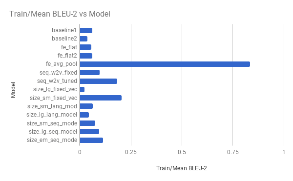
Bar Chart of Experiment vs Model Skill on the Training Dataset
Results on the test dataset:

Bar Chart of Experiment vs Model Skill on the Test Dataset
From just looking at the mean results on the test dataset, we can suggest:
- Perhaps pooling is not required after the photo feature extractor (fe_flat at 0.135231).
- Perhaps average pooling offers an advantage over max pooling after the photo feature extractor (fe_avg_pool at 0.060847).
- Perhaps a smaller sized fixed-length vector after the sub-models is a good idea (size_sm_fixed_vec at 0.063148).
- Perhaps adding more layers to the language model offers some benefit (size_lg_lang_model at 0.067658).
- Perhaps adding more layers to the sequence model offers some benefit (size_lg_seq_model at 0.09697).
I would also recommend exploring combinations of these suggestions.
We can also review the distribution of results.
Below is some code to load the saved results from each experiment and create a box-and-whisker plot of results on the train and test sets for review.
|
1 2 3 4 5 6 7 8 9 10 11 12 13 14 15 16 17 18 19 20 21 22 23 |
from os import listdir from pandas import read_csv from pandas import DataFrame from matplotlib import pyplot # load all .csv results into a dataframe train, test = DataFrame(), DataFrame() directory = 'results' for name in listdir(directory): if not name.endswith('csv'): continue filename = directory + '/' + name data = read_csv(filename, header=0) experiment = name.split('.')[0] train[experiment] = data['train'] test[experiment] = data['test'] # plot results on train train.boxplot(vert=False) pyplot.show() # plot results on test test.boxplot(vert=False) pyplot.show() |
Distribution of results on the training dataset.

Box and Whisker Plot of Experiment vs Model Skill on the Training Dataset
Distribution of results on the test dataset.
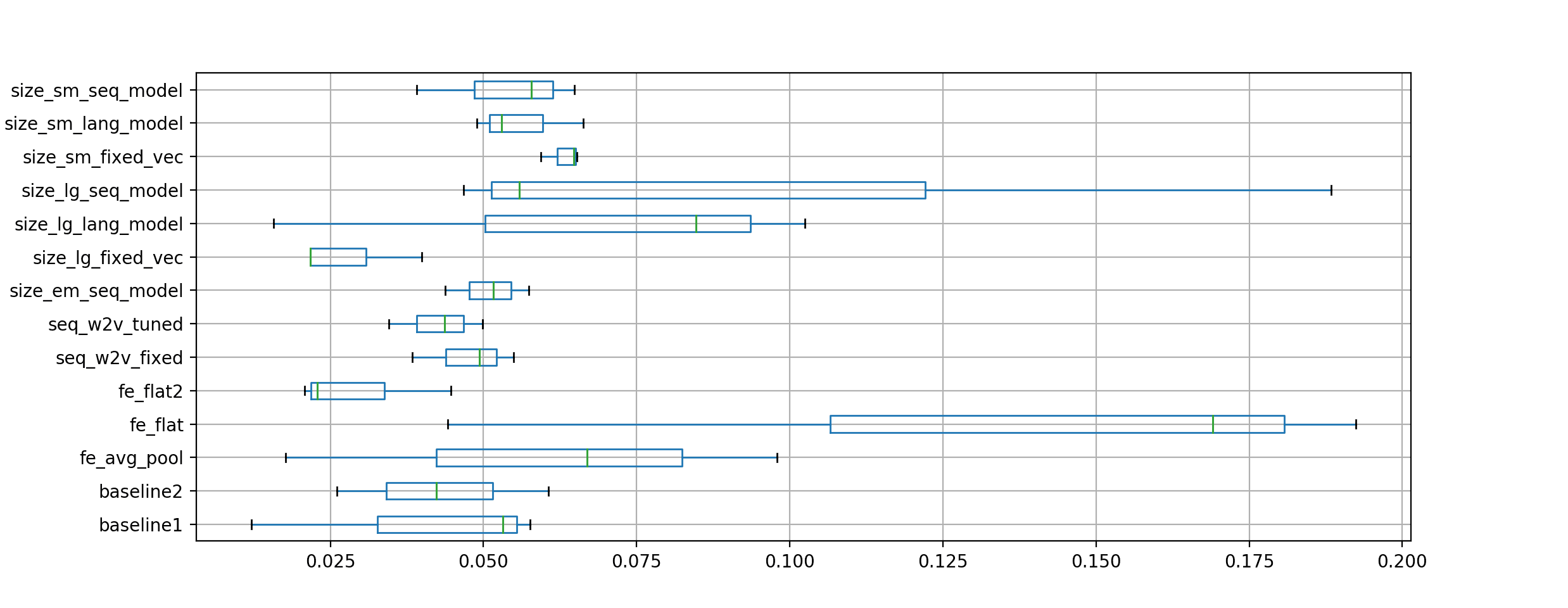
Box and Whisker Plot of Experiment vs Model Skill on the Test Dataset
A review of these distributions suggests:
- The spread on the flat results is large; perhaps going with average pooling might be safer.
- The spread on the larger language model is large and skewed in the wrong/risky direction.
- The spread on the larger sequence model is large and skewed in the right direction.
- There may be some benefit in a smaller fixed-length vector size.
I would expect increasing repeats to 5, 10, or 30 would tighten up these distributions somewhat.
Further Reading
This section provides more resources on the topic if you are looking go deeper.
Papers
- Show and Tell: A Neural Image Caption Generator, 2015.
- Show, Attend and Tell: Neural Image Caption Generation with Visual Attention, 2016.
- Network In Network, 2013.
Related Captioning Projects
- caption_generator: An image captioning project
- Keras Image Caption
- Neural Image Captioning (NIC)
- Keras deep learning for image caption retrieval
- DataLab Cup 2: Image Captioning
Other
API
Summary
In this tutorial, you discovered how you can use a small sample of the photo captioning dataset to explore different model designs.
Specifically, you learned:
- How to prepare data for photo captioning modeling.
- How to design a baseline and test harness to evaluate the skill of models and control for their stochastic nature.
- How to evaluate properties like model skill, feature extraction model, and word embeddings in order to lift model skill.
What experiments can you think up?
What else have you tried?
What are the best results you can get on the train and test dataset?
Let me know in the comments below.
Develop Deep Learning models for Text Data Today!
Develop Your Own Text models in Minutes
...with just a few lines of python code
Discover how in my new Ebook:
Deep Learning for Natural Language Processing
It provides self-study tutorials on topics like:
Bag-of-Words, Word Embedding, Language Models, Caption Generation, Text Translation and much more...
Finally Bring Deep Learning to your Natural Language Processing Projects
Skip the Academics. Just Results.


Hats off, another ace tutorial!
I’m curious how the TimeDistributed layer impacts the data before the concatenation. Is it possible to skip it? Also, is there a reason you are using VGG instead of the InceptionResNetV2 class other than memory/compute constraints.
Thanks!
I chose VGG because it is smaller and simpler. You can use anything you wish.
You can skip the TimeDistributed as Dense can support time steps now I believe. I like it in there as it reminds me what is going on (e.g. outputting time steps).
Ho jason, why don t you reset the LSTM states between the inputs related to different images? Ad they are not related to the same sequences.
For speed of training.
It’s a great suggestion though, try it and see if it lifts skill! Let me know how you go.
Thanks! In order to try this way, should I set stateful=True (avoiding the LSTM to reset itself automatically) and manually run model.reset_states() before training a single batch? (each batch is related to the sequence of a single image).
Yes.
What’s the logic of the +1 when you are creating the vocab len: “vocab_size = len(tokenizer.word_index) + 1”? Is it to leave remove for the 0?
Thanks
Good question, to make space for 0 – words in the vocab start at 1.
Does it mean we leave index 0 for ‘endseq’ token?
No, the start and end tokens are legit parts of the problem. The model must specify when the sequence has ended.
i got a error : Error when checking input: expected input_11 to have 4 dimensions, but got array with shape (28, 4096)
Are you able to confirm that your libraries are up to date and that you copied all of the code from the post?
This happens to me as well. But this is when I try to use the pretrained word2vec with the initially defined data generator etc code. I am trying to see what modifications would allow the pretrained word2vec to run
can i get the code in github?
The code is on the post, why do you need it on github?
Hello Jason.
Thank you very much for your article.
I have a practical question regarding training an encoder decoder network.
So basically I have images of serial numbers and I want to predict the full serial number. (E.G 018F6176)
So if I train a network to predict the next character I would practically have to create a for loop predicting untill I reach max length or the stop word.
This I get. However how can i structure my data?
What I have is the following
data is a numpy float array of shape (nb_samples width, height, nb_channels=3,).
labels is a numpy integer array of shape (nb_samples, max_caption_len)
So if I were to construct a similar dataset with the structure you get from create_sequences() my number of samples would increase and how do I ensure that images are loaded so as the sequence for each images comes in the correct order(or does that matter?)
Hopefully this makes sense to you.
Best regards
Niels
Great question.
The caption model is the approach you want to use I believe.
See this post, specifically the section titled “ord-By-Word Model”:
https://machinelearningmastery.com/prepare-photo-caption-dataset-training-deep-learning-model/
It will show you exactly how to prepare your data and how to think about it.
Thank you. This is exactly what I was looking for. One question though. Does the order of input matter, so let’s say all samples for image 1 comes in order, all samples for image 2 next etc.
Because then I would have to create a batch generator, however I would like to avoid that.
My initial thought is it doesn’t really matter since you are just training the algorithm to recognize what comes next regarding previous input. Is that a correct assumption?
Best Regards
Niels
I think so, I think all samples for a give photo should be together by intuition (LSTMs have memory across the batch), but testing all assumptions is a good idea.
Okay. I created a model both with the data_generator and randomly splitting in train,test(image order scrambled). The tran, test model did not seem to converge(max 17% validation accuracy). However the data_generator model(where order is preserved) reaches 99.5% validation accuracy , so that’s pretty awesome.
Thank you for your time ????
Very nice. Thanks for running the experiment!
Why and How the dimension of input_1 is (7, 7, 512)
That is the shape that we saved the extracted features from the photos.
Thanks for your tutorials, Jason. I can run this tutorial in contrary with the tutorial on the same dataset https://machinelearningmastery.com/develop-a-deep-learning-caption-generation-model-in-python/ where memory errors occur.
I compared both examples and found that the feature extraction of the images is different. This example the features are a 3-dimensional array with the shape (7, 7, 512) the other example the result is a 1-dimensional 4,096 element vector. The features.pkl file of this experiment is much larger compared to the other example. What is the reason of the different shape of the features?
Perhaps the VGG model is cut at different points? e.g. keeping the dense or discarding it and working with the CNN outputs. I don’t recall, but a comparison of the code would make it clearer.
Thanks for the tutorial, Jason. Here you are using features from a pretrained cnn model. But I want to backpropagate the error through the cnn as well and hence jointly train the cnn and lstm. i.e. load the cnn through a pretrained model and than train it further. Can you suggest a way to do that? Thanks.
Yes, you can load the CNN as part of your in memory model.
Hello Jason,
Thanks for this great posts and the one in here (https://machinelearningmastery.com/develop-a-deep-learning-caption-generation-model-in-python/)!!
I was trying to run the example you posted in here.I was able to train using different learning rate and more epoch on your “average pooling” model and saved them in a .h5 file.
However when I try to use the code in (https://machinelearningmastery.com/develop-a-deep-learning-caption-generation-model-in-python/) to Generate New Captions with the “Average Model” I trained, I got this error:
ValueError: Error when checking : expected input_1 to have 4 dimensions, but got array with shape (1, 4096)
Just wonder do you know how to use this .h5 file i just trained to make prediction on one other photo? Thanks!!
It looks like your photo features might have too many dimensions. Change your code to provide the photo pixels directly. e.g.: photo[0]
Hai Jason,
that’s a great post. Really it is very helpful for me. However, I get the following error:
File “”, line 1, in
runfile(‘C:/Users/33083707/Codes/Projects/Final.py’, wdir=’C:/Users/33083707/Codes/Projects’)
File “C:\Users\33083707\Anaconda3\lib\site-packages\spyder\utils\site\sitecustomize.py”, line 866, in runfile
execfile(filename, namespace)
File “C:\Users\33083707\Anaconda3\lib\site-packages\spyder\utils\site\sitecustomize.py”, line 102, in execfile
exec(compile(f.read(), filename, ‘exec’), namespace)
File “C:/Users/33083707/Codes/Projects/Final.py”, line 244, in
test_score = evaluate_model(model, test_descriptions, test_features, tokenizer, max_length)
File “C:/Users/33083707/Codes/Projects/Final.py”, line 202, in evaluate_model
bleu = corpus_bleu(actual, predicted)
File “C:\Users\33083707\Anaconda3\lib\site-packages\nltk\translate\bleu_score.py”, line 146, in corpus_bleu
p_i = modified_precision(references, hypothesis, i)
File “C:\Users\33083707\Anaconda3\lib\site-packages\nltk\translate\bleu_score.py”, line 287, in modified_precision
return Fraction(numerator, denominator, _normalize=False)
File “C:\Users\33083707\Anaconda3\lib\fractions.py”, line 186, in __new__
raise ZeroDivisionError(‘Fraction(%s, 0)’ % numerator)
ZeroDivisionError: Fraction(0, 0)
Sorry to hear that, I have some suggestions to try here:
https://machinelearningmastery.com/faq/single-faq/why-does-the-code-in-the-tutorial-not-work-for-me
Hello Dr. Jason,
I want to try this on my own data, but I don’t know how to prepare it. I have a folder of images and a CSV file. Each line in the csv file contains an image ID/name and a caption that describes the image. Any advice on how to proceed?
Thank you
Start by writing code to load the images into memory.
Perhaps you can use PIL or Pillo to load the images?
in the following part of the code :
# run experiment
train_results, test_results = list(), list()
for i in range(n_repeats):
# define the model
model = define_model(vocab_size, max_length)
# fit model
model.fit_generator(data_generator(train_descriptions, train_features, tokenizer, max_length, n_photos_per_update), steps_per_epoch=n_batches_per_epoch, epochs=n_epochs, verbose=verbose)
# evaluate model on training data
train_score = evaluate_model(model, train_descriptions, train_features, tokenizer, max_length)
test_score = evaluate_model(model, test_descriptions, test_features, tokenizer, max_length)
# store
train_results.append(train_score)
test_results.append(test_score)
print(‘>%d: train=%f test=%f’ % ((i+1), train_score, test_score))
why are you defining the model within the for loop ? shouldn’t it be defined outside of it ?
Nope, I want a new model (random weights) for each repeat.
Why would I define outside the loop?
Could you please explain why is that? I think that a model has to be defined, and the weights are to be trained by learning from examples. But defining a new model everytime would delete the previously learned weights. Where am I going wrong?
Yes, we want to throw it away. We are repeating the experiment with a model each time so we can see how well the model on our data performs on average. Not the performance of any one randomly fit model.
You can learn more here:
https://machinelearningmastery.com/evaluate-skill-deep-learning-models/
Hi Jason, Thank you very much.
I tried to use DenseNet-121 model instead of VGG16 model to extract the features. But I got an error like:
ValueError: Error when checking input: expected input_1 to have 4 dimensions, but got array with shape (21, 1024).
Can you please suggest me anything about this.
This is because both the CNN models have different output dimensions of their last layer from where you are pulling the features for your images. Best guess is to convert the output dimension of your DenseNet model into the same dimension of that of VGG-16.
Also, if you use Flatten() instead of GlobalMaxPooling2D() then I guess you will not face the same problem.
Not really, I don’t know about the things you are trying.
Hi Jason
Thanks for the wonderful tutorial as always
I got this result on 70 epochs and 3 repeats
it seems that the accuracy increases when we have a large number of epochs
but I don’t understand why I got the train and test = 0
this is my result
Epoch 70/70
– 14s – loss: 1.8873 – acc: 0.4100
Actual: startseq child and woman are at waters edge in big city endseq
Predicted: startseq child woman are edge edge in big endseq
Actual: startseq boy with stick kneeling in front of goalie net endseq
Predicted: startseq boy boy in in front and and and of of of of of in front and of of in front boy front and of of
Actual: startseq woman crouches near three dogs in field endseq
Predicted: startseq two dog dogs in near near near near near near near near near near near near near near near near near near near near near
Actual: startseq boy bites hard into treat while he sits outside endseq
Predicted: startseq boy bites sits while while outside endseq
Actual: startseq person eats takeout while watching small television endseq
Predicted: startseq person eats while takeout small small television endseq
Actual: startseq couple with young child wrapped in blanket sitting on concrete step endseq
Predicted: startseq boy girls in in in bike endseq
Actual: startseq adults and children stand and play in front of steps near wooded area endseq
Predicted: startseq boy and young boy and and and and and and and and and and and and and and and and and and and and and
Actual: startseq boy in grey pajamas is jumping on the couch endseq
Predicted: startseq boy man into if rough endseq
Actual: startseq boy holding kitchen utensils and making threatening face endseq
Predicted: startseq girl holds shorts shorts shorts with down her endseq
Actual: startseq man in green hat is someplace up high endseq
Predicted: startseq boy in with with waves endseq
>3: train=0.000000 test=0.000000
train test
count 3.000000e+00 3.000000e+00
mean 6.038250e-02 4.013559e-155
std 1.045856e-01 2.160777e-156
min 2.413005e-78 3.808820e-155
25% 2.799294e-78 3.900627e-155
50% 3.185584e-78 3.992435e-155
75% 9.057374e-02 4.115929e-155
max 1.811475e-01 4.239423e-155
Also, I got this warning
UserWarning:
The hypothesis contains 0 counts of 3-gram overlaps.
Therefore the BLEU score evaluates to 0, independently of
how many N-gram overlaps of lower order it contains.
Consider using lower n-gram order or use SmoothingFunction()
warnings.warn(_msg)
would you mind giving your opinion on my experiment and suggesting a better solution for the warning?
Thanks
Nice work!
BLEU may give warnings when some predictions are shorter than expected. This might help understand the BLEU score calculation some more:
https://machinelearningmastery.com/calculate-bleu-score-for-text-python/
what is the highest accuracy that has been achieved for a image captioning model?
We don’t measure accuracy, instead we measure perplexity or bleu scores.
The best score will depend on the specific benchmark dataset used.
hi jason .. your posts are good .
but i am not able to get accuracy above 0.3.
I tried increasing epochs also. but no change in accuracy.
can you please help in increase accuracy to atleast 0.7 or 0.8
I don’t recommend using accuracy for caption generation, instead use bleu score or perplexity.
I have general advice for improving deep learning models here:
https://machinelearningmastery.com/start-here/#better
Hi Jason! I can’t download dataset. Framing_Image_Description. 404 Not Found
Thanks, I have added a direct link to the dataset.
Hi Sir, I have seen your blog “How to Develop a Deep Learning Photo Caption Generator from Scratch”. In that tutorial you have not used RepeatVector and TimeDistributed function. In this tutorial you used both function. As I am new in Deep learning. Can you please help me out by explaining the use of RepeatVector and TimeDistributed function. What if we did not applied this function, will it affect our model performance ?
Thanks,
Ankit
You can choose any model architecture you wish. There is no one best model.
Perhaps one the one from the other post or one of your own devising, or test both and see what works best for you?
great tutorial jason! i would ask one thing about CNN? what Window size has been used by the CNN in the tutorial?
What do you mean by window size exactly?
what else can be tried to further improve BLEU scores?
I have some suggestions here:
https://machinelearningmastery.com/improve-deep-learning-performance/
my pyplot library is not working properly.please provide a detailed tutorial about installing and setup of pyplot library in python as well.thanks in advance
Perhaps just comment put the plot_model lines for now?
what does n_repeats = 3 means? i mean to say what if i pass the n_repeats = 1? what will be the difference of passing two different repeats?
The number of times that the experiment is repeated from which the results are averaged.
More repeats will give a better idea of the expected performance of the method.
can the change of CNN architecture can improve BLUE scores??
secondly how can i interpret these results??please give in depth overview..which scores should be high for better model performances
>3: train=0.000000 test=0.000000
train test
count 3.000000e+00 3.000000e+00
mean 1.219064e-78 3.030008e-155
std 2.247343e-79 8.613845e-156
min 1.078167e-78 2.152162e-155
25% 1.089478e-78 2.608047e-155
50% 1.100788e-78 3.063932e-155
75% 1.289512e-78 3.468930e-155
max 1.478235e-78 3.873929e-155
Perhaps try some changes and compare the results?
Jason i have some questions in my mind .Please make it a bit clear.
In the “Size of fixed length Vector” part of the tutorial.
fe2 = Dense(64/128/256, activation=’relu’)(fe1)
1)What does 64/128/256 is representing ?Is it photo features vectors or something else?
2)how and why we can increase or decrease a vector of features?
3)the output in this case of VGG16 is 4096 dimensional vector..then where we are giving that (image)feature as input to the model?
3)why we are taking the multiples of 64? why we can’t take randomly ?
It is the number of nodes in the layer.
What do you mean by increase/decrease vector of features? Do you mean the length of the feature vector of the photo? If so, perhaps test using different pre-trained models.
The feature vector is X1, perhaps re-read the tutorial?
Multiples of 64 is common for nodes in the model, no good reason.
so ,can we change thr number of nodes in vgg16?if yes then explain in which layer of vgg16 the nodes are changing??
secondly let me know that are we using validation set in experiment or not?
You either have specified for a validation dataset to be used or not.
Perhaps I don’t understand your question?
Yes, but you will then need to refit the model.
my question is just that we are changing the number of nodes from 128 to 64/256 of which layer of vgg16?
vgg_16 has 16 layer right..so which layer nodes are changing in this tutorial?
If you want to change the number of layers or number of nodes in a layer, go for it.
We do not make those changes in this tutorial. For more on changing nodes and layers, see this tutorial:
https://machinelearningmastery.com/how-to-control-neural-network-model-capacity-with-nodes-and-layers/
secondly have we used different validation and testing datsets in the tutorial??if not then how to do that
Yes, we use different datasets for train and test, more on the distinction here:
https://machinelearningmastery.com/difference-test-validation-datasets/
how can i let it know that my training is the right one??i mean to say that how can i confirm that my model is learning well..
Evaluate it using a robust test harness, like k-fold cross validation.
Or a large train/test split.
how can i use k-fold cross validation?do you have any tutorial so i can get idea from that
This will help:
https://machinelearningmastery.com/k-fold-cross-validation/
my blue scores on test dataset is resulting low value that approaches to zero.What mistakes i am doing in my training? my mean train is 0.194386 while my test mean score is 0.01468624
Perhaps your model is overfitting the training dataset?
Perhaps try a smaller learning rate or stop training sooner or similar?
how can i update the current code of the tutorial so that i can make K-folds(cross validation) of my dataset and then evaluate the performance of my model on that base(so that to ensure low or no bias)
Perhaps this will help:
https://machinelearningmastery.com/k-fold-cross-validation/
In the previous post you have taken one-dimensional image features of shape 4096,while in this post you are taking 3-dimensional image features of shape (7,7,512)…why??? whats the difference in these two different features? are these both are VGG features but both of different layers???
The linked post introduces k-fold cross-validation in the most general sense.
please check my question once again..i am asking about image deatures dimension…not about k-fold
Hello Jason,
When I apply your code, this part:
I get “NotImplementedError: Cannot convert a symbolic Tensor (args_2:0) to a numpy array.”
I am not sure how to solve the problem. Would you help me solve it?
Thank you.
Sorry to hear that, this will help:
https://machinelearningmastery.com/faq/single-faq/why-does-the-code-in-the-tutorial-not-work-for-me
It worked when I tried it with downgraded Tensorflow (1.14) from 2.1. What I mean is the code worked without the error notification. But I am not sure if it works completely fine. Because the result does not provide me appended train_results and test_results. It is just blank. As it is a for-loop, it should work repetitively and the results should be appended accordingly. I checked ur suggestion for checking and I believe I did all.
Any clue why wouldn’t it work smoothly?
Thank you.
Are you running from the command line (not a notebook or ide):
https://machinelearningmastery.com/faq/single-faq/how-do-i-run-a-script-from-the-command-line