The introduction of GPT-3, particularly its chatbot form, i.e. the ChatGPT, has proven to be a monumental moment in the AI landscape, marking the onset of the generative AI (GenAI) revolution. Although prior models existed in the image generation space, it’s the GenAI wave that caught everyone’s attention.
Stable Diffusion is a member of the GenAI family for image generation. It is known for its possibility to customization, freely available to run on your own hardware, and actively improving. It is not the only one. For example, OpenAI released DALLE-3 as part of its ChatGPTPlus subscription to allow image generation. But Stable Diffusion showed remarkable success in generating images from text as well as from other existing images. The recent integration of video generation capabilities into diffusion models provides a compelling case for studying this cutting-edge technology.
In this post, you will learn some technical details of Stable Diffusion and how to set it up on your own hardware.
Let’s get started.
A Technical Introduction to Stable Diffusion Photo by Denis Oliveira. Some rights reserved.
Overview
This post is in four parts; they are:
How Do Diffusion Models Work
Mathematics of Diffusion Models
Why Is Stable Diffusion Special
How to Install Stable Diffusion WebUI
How Do Diffusion Models Work
To understand diffusion models, let us first revisit how image generation using machines was performed before the introduction of Stable Diffusion or its counterparts today. It all started with GANs (Generative Adversarial Networks), wherein two neural networks engage in a competitive and cooperative learning process.
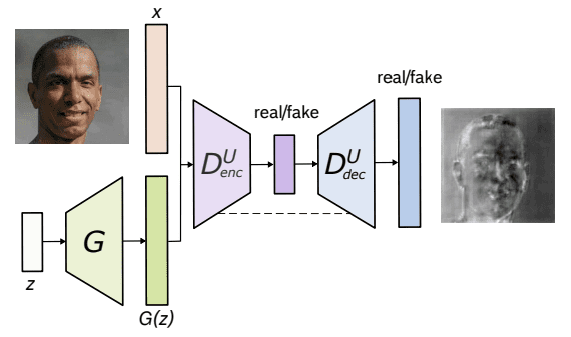
The first one is the generator network, which fabricates synthetic data, in this case, images, that are indistinguishable from real ones. It produces random noise and progressively refines it through several layers to generate increasingly realistic images.
The second network, i.e., the discriminator network, acts as the adversary, scrutinizing the generated images to differentiate between real and synthetic ones. Its goal is to accurately classify images as either real or fake.
Architecture of U-Net GAN. From Schonfeld et al. (2020)
The diffusion models assume that a noisy image or pure noise is an outcome of repeated overlay of noise (or Gaussian Noise) on the original image. This process of noise overlay is called the Forward Diffusion. Now, exactly opposite to this is the Reverse Diffusion, which involves going from a noisy image to a less noisy image, one step at a time.
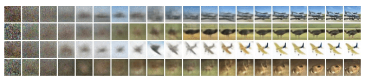
Below is an illustration of the Forward Diffusion process from right to left, i.e., clear to noisy image.
Diffusion process. Image from Ho et al. (2020)
Mathematics of Diffusion Models
Both the Forward and Reverse Diffusion processes follow a Markov Chain, which means that at any time step t, the pixel value or noise in an image depends only on the previous image.
Forward Diffusion
Mathematically, each step in the forward diffusion process can be represented using the below equation:
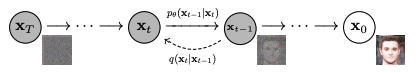
where $q(x_t\mid x_{t-1})$ is a normal distribution with mean $\mu_t = \sqrt{1-\beta_t}x_{t-1}$ and variance $\Sigma_t = \beta_t \mathbb{I}$, and $\mathbf{I}$ is the identity matrix, images (as a latent variable) in each step $\mathbf{x}_t$ is a vector, and the mean and variance are parameterized by the scalar value $\beta_t$.
Forward diffusion $q(\mathbf{x}_t\mid\mathbf{x}_{t-1})$ and reverse diffusion $p_\theta(\mathbf{x}_{t-1}\mid\mathbf{x}_t)$. Figure from Ho et al. (2020)
The posterior probability of all the steps in the forward diffusion process is thus defined below:
Reverse diffusion, which is the opposite of the forward diffusion process, works similarly. While the forward process maps the posterior probability given the prior probability, the reverse process does the opposite, i.e., maps the prior probability given the posterior one.
where $p_\theta$ applies reverse diffusion, also called the trajectory.
As the time step $t$ approaches infinity, the latent variable $\mathbf{x}_T$ tends to an almost isotropic Gaussian distribution (i.e., purely noise with no image content). The aim is to learn $q(\mathbf{x}_{t-1}\mid \mathbf{x}_t)$, where the process starts at the sample from $\mathcal{N}(0,\mathbf{I})$ called $\mathbf{x}_T$. We run the complete reverse process, one step at a time, to reach a sample from $q(\mathbf{x}_0)$, i.e., the generated data from the actual data distribution. In layman’s term, the reverse diffusion is to create an image out of random noise in many small steps.
Why Is Stable Diffusion Special?
Instead of directly applying the diffusion process to a high-dimensional input, Stable diffusion projects the input into a reduced latent space using an encoder network (that is where the diffusion process occurs). The rationale behind this approach is to reduce the computational load involved in training diffusion models by handling the input within a lower-dimensional space. Subsequently, a conventional diffusion model (such as a U-Net) is used to generate new data, which are then upsampled using a decoder network.
How to Install Stable Diffusion WebUI?
You can use stable diffusion as a service by subscription, or you can download and run on your computer. There are two major ways to use it on your computer: The WebUI and the CompfyUI. Here you will be shown to install WebUI.
Note: Stable Diffusion is compute heavy. You may need a decent hardware with supported GPU to run at a reasonable performance.
The Stable Diffusion WebUI package for Python programming language is free to download and use from its GitHub page. Below are the steps to install the library on an Apple Silicon chip, where other platform are mostly the same as well:
Prerequisites. One of the prerequisites to the process is having a setup to run the WebUI. It is a Python-based web server with the UI built using Gradio. The setup is mostly automatic, but you should make sure some basic components are available, such as git and wget. When you run the WebUI, a Python virtual environment will be created.
In macOS, you may want to install a Python system using Homebrew because some dependencies may need a newer version of Python than what the macOS shipped by default. See the Homebrew’s setup guide. Then you can install Python with Homebrew using:
This will create a folder named stable-diffusion-webui and you should work in this folder for the following steps.
Checkpoints. The WebUI is to run the pipeline but the Stable Diffusion model is not included. You need to download the model (also known as checkpoints), and there are several versions you can choose from. These can be downloaded from various sources, most commonly from HuggingFace. The following section will cover this step in more detail. All Stable Diffusion models/checkpoints should be placed in the directory stable-diffusion-webui/models/Stable-diffusion.
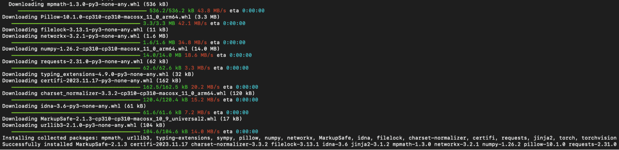
First run. Navigate into the stable-diffusion-webui directory using the command line and run ./webui.sh to launch the web UI. This action will create and activate a Python virtual environment using venv, automatically fetching and installing any remaining required dependencies.
Python modules installed during the first run of WebUI
Subsequent run. For future access to the web UI, re-run ./webui.sh at the WebUI directory. Note that the WebUI doesn’t update itself automatically; to update it, you have to execute git pull before running the command to ensure you’re using the latest version. What this webui.sh script does is to start a web server, which you can open up your browser to access to the Stable Diffusion. All the interaction should be done over the browser, and you can shutdown the WebUI by shutting down the web server (e.g., pressing Control-C on the terminal running webui.sh).
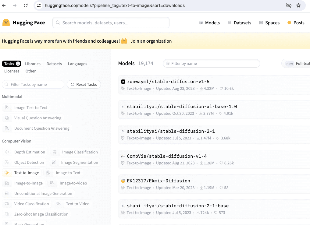
You can download Stable Diffusion models via Hugging Face by selecting a model of interest and proceeding to the “Files and versions” section. Look for files labeled with the “.ckpt” or “.safetensors” extensions and click the right-facing arrow next to the file size to initiate the download. SafeTensor is an alternative format to Python’s pickle serialization library; their difference is handled by the WebUI automatically, so you can consider them equivalent.
There are several models from Hugging Face if you search by the model name “stable-diffusion”.
Several official Stable Diffusion models that we may use in the upcoming chapters include:
A model and configuration file are essential for Stable Diffusion versions 2.0 and 2.1. Additionally, when generating images, ensure the image width and height are set to 768 or higher:
Stable Diffusion 2.0 (768-v-ema.ckpt)
Stable Diffusion 2.1 (v2-1_768-ema-pruned.ckpt)
The configuration file can be found on GitHub at the following location:
After you downloaded v2-inference-v.yaml from above, you should place it in the same folder as the model matching the model’s filename (e.g., if you downloaded the 768-v-ema.ckpt model, you should rename this configuration file to 768-v-ema.yaml and store it in stable-diffusion-webui/models/Stable-diffusion along with the model).
A Stable Diffusion 2.0 depth model (512-depth-ema.ckpt) also exists. In that case, you should download the v2-midas-inference.yaml configuration file from:
and save it to the model’s folder as stable-diffusion-webui/models/Stable-diffusion/512-depth-ema.yaml. This model functions optimally at image dimensions of 512 width/height or higher.
Another location that you can find model checkpoints for Stable Diffusion is https://civitai.com/, which you can see the samples as well.
Further Readings
Below are several papers that are referenced above:
“Denoising Diffusion Probabilistic Models” by Ho, Jain, and Abbeel (2020). arXiv 2006.11239
Summary
In this post, we learned the fundamentals of diffusion models and their broad application across diverse fields. In addition to expanding on the recent successes of their image and video generation successes, we discussed the Forward and Reverse Diffusion processes and modeling posterior probability.
Stable Diffusion’s unique approach involves projecting high-dimensional input into a reduced latent space, reducing computational demands via encoder and decoder networks.
Moving forward, we’ll learn the practical aspects of generating images using Stable Diffusion WebUI. Our exploration will cover model downloads and leveraging the web interface for image generation.


No comments yet.