
Time series is different from more traditional classification and regression predictive modeling problems.
The temporal structure adds an order to the observations. This imposed order means that important assumptions about the consistency of those observations needs to be handled specifically.
For example, when modeling, there are assumptions that the summary statistics of observations are consistent. In time series terminology, we refer to this expectation as the time series being stationary.
These assumptions can be easily violated in time series by the addition of a trend, seasonality, and other time-dependent structures.
In this tutorial, you will discover how to check if your time series is stationary with Python.
After completing this tutorial, you will know:
- How to identify obvious stationary and non-stationary time series using line plot.
- How to spot check summary statistics like mean and variance for a change over time.
- How to use statistical tests with statistical significance to check if a time series is stationary.
Kick-start your project with my new book Time Series Forecasting With Python, including step-by-step tutorials and the Python source code files for all examples.
Let’s get started.
- Updated Feb/2017: Fixed typo in interpretation of p-value, added bullet points to make it clearer.
- Updated May/2018: Improved language around reject vs fail to reject of statistical tests.
- Updated Apr/2019: Updated the link to dataset.
- Updated Aug/2019: Updated data loading to use new API.
- Updated Nov/2019: Updated mean/variance example for Python 3, also updated bug in data loading (thanks John).

How to Check if Time Series Data is Stationary with Python
Photo by Susanne Nilsson, some rights reserved.
Stationary Time Series
The observations in a stationary time series are not dependent on time.
Time series are stationary if they do not have trend or seasonal effects. Summary statistics calculated on the time series are consistent over time, like the mean or the variance of the observations.
When a time series is stationary, it can be easier to model. Statistical modeling methods assume or require the time series to be stationary to be effective.
Below is an example of loading the Daily Female Births dataset that is stationary.
|
1 2 3 4 5 |
from pandas import read_csv from matplotlib import pyplot series = read_csv('daily-total-female-births.csv', header=0, index_col=0) series.plot() pyplot.show() |
Running the example creates the following plot.
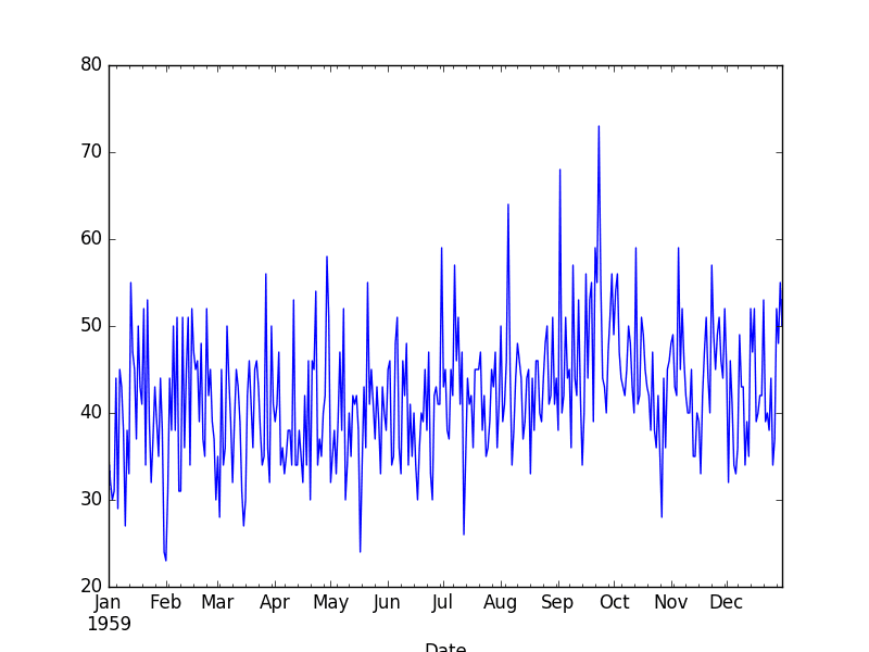
Daily Female Births Dataset Plot
Stop learning Time Series Forecasting the slow way!
Take my free 7-day email course and discover how to get started (with sample code).
Click to sign-up and also get a free PDF Ebook version of the course.
Non-Stationary Time Series
Observations from a non-stationary time series show seasonal effects, trends, and other structures that depend on the time index.
Summary statistics like the mean and variance do change over time, providing a drift in the concepts a model may try to capture.
Classical time series analysis and forecasting methods are concerned with making non-stationary time series data stationary by identifying and removing trends and removing seasonal effects.
Below is an example of the Airline Passengers dataset that is non-stationary, showing both trend and seasonal components.
|
1 2 3 4 5 |
from pandas import read_csv from matplotlib import pyplot series = read_csv('international-airline-passengers.csv', header=0, index_col=0) series.plot() pyplot.show() |
Running the example creates the following plot.
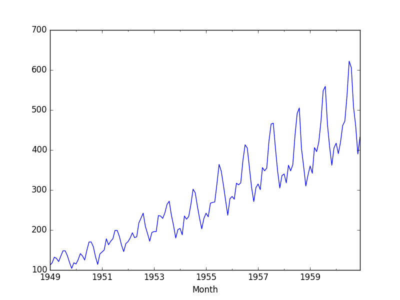
Non-Stationary Airline Passengers Dataset
Types of Stationary Time Series
The notion of stationarity comes from the theoretical study of time series and it is a useful abstraction when forecasting.
There are some finer-grained notions of stationarity that you may come across if you dive deeper into this topic. They are:
They are:
- Stationary Process: A process that generates a stationary series of observations.
- Stationary Model: A model that describes a stationary series of observations.
- Trend Stationary: A time series that does not exhibit a trend.
- Seasonal Stationary: A time series that does not exhibit seasonality.
- Strictly Stationary: A mathematical definition of a stationary process, specifically that the joint distribution of observations is invariant to time shift.
Stationary Time Series and Forecasting
Should you make your time series stationary?
Generally, yes.
If you have clear trend and seasonality in your time series, then model these components, remove them from observations, then train models on the residuals.
If we fit a stationary model to data, we assume our data are a realization of a stationary process. So our first step in an analysis should be to check whether there is any evidence of a trend or seasonal effects and, if there is, remove them.
— Page 122, Introductory Time Series with R.
Statistical time series methods and even modern machine learning methods will benefit from the clearer signal in the data.
But…
We turn to machine learning methods when the classical methods fail. When we want more or better results. We cannot know how to best model unknown nonlinear relationships in time series data and some methods may result in better performance when working with non-stationary observations or some mixture of stationary and non-stationary views of the problem.
The suggestion here is to treat properties of a time series being stationary or not as another source of information that can be used in feature engineering and feature selection on your time series problem when using machine learning methods.
Checks for Stationarity
There are many methods to check whether a time series (direct observations, residuals, otherwise) is stationary or non-stationary.
- Look at Plots: You can review a time series plot of your data and visually check if there are any obvious trends or seasonality.
- Summary Statistics: You can review the summary statistics for your data for seasons or random partitions and check for obvious or significant differences.
- Statistical Tests: You can use statistical tests to check if the expectations of stationarity are met or have been violated.
Above, we have already introduced the Daily Female Births and Airline Passengers datasets as stationary and non-stationary respectively with plots showing an obvious lack and presence of trend and seasonality components.
Next, we will look at a quick and dirty way to calculate and review summary statistics on our time series dataset for checking to see if it is stationary.
Summary Statistics
A quick and dirty check to see if your time series is non-stationary is to review summary statistics.
You can split your time series into two (or more) partitions and compare the mean and variance of each group. If they differ and the difference is statistically significant, the time series is likely non-stationary.
Next, let’s try this approach on the Daily Births dataset.
Daily Births Dataset
Because we are looking at the mean and variance, we are assuming that the data conforms to a Gaussian (also called the bell curve or normal) distribution.
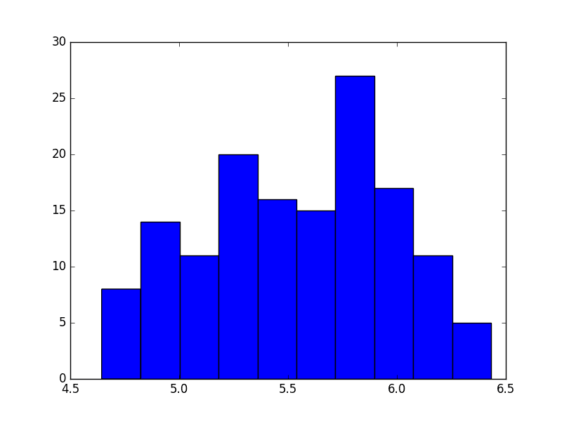
We can also quickly check this by eyeballing a histogram of our observations.
|
1 2 3 4 5 |
from pandas import read_csv from matplotlib import pyplot series = read_csv('daily-total-female-births.csv', header=0, index_col=0) series.hist() pyplot.show() |
Running the example plots a histogram of values from the time series. We clearly see the bell curve-like shape of the Gaussian distribution, perhaps with a longer right tail.
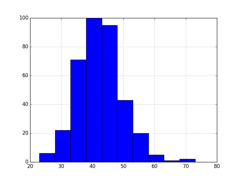
Histogram of Daily Female Births
Next, we can split the time series into two contiguous sequences. We can then calculate the mean and variance of each group of numbers and compare the values.
|
1 2 3 4 5 6 7 8 9 |
from pandas import read_csv series = read_csv('daily-total-female-births.csv', header=0, index_col=0) X = series.values split = round(len(X) / 2) X1, X2 = X[0:split], X[split:] mean1, mean2 = X1.mean(), X2.mean() var1, var2 = X1.var(), X2.var() print('mean1=%f, mean2=%f' % (mean1, mean2)) print('variance1=%f, variance2=%f' % (var1, var2)) |
Running this example shows that the mean and variance values are different, but in the same ball-park.
|
1 2 |
mean1=39.763736, mean2=44.185792 variance1=49.213410, variance2=48.708651 |
Next, let’s try the same trick on the Airline Passengers dataset.
Airline Passengers Dataset
Cutting straight to the chase, we can split our dataset and calculate the mean and variance for each group.
|
1 2 3 4 5 6 7 8 9 |
from pandas import read_csv series = read_csv('international-airline-passengers.csv', header=0, index_col=0) X = series.values split = len(X) / 2 X1, X2 = X[0:split], X[split:] mean1, mean2 = X1.mean(), X2.mean() var1, var2 = X1.var(), X2.var() print('mean1=%f, mean2=%f' % (mean1, mean2)) print('variance1=%f, variance2=%f' % (var1, var2)) |
Running the example, we can see the mean and variance look very different.
We have a non-stationary time series.
|
1 2 |
mean1=182.902778, mean2=377.694444 variance1=2244.087770, variance2=7367.962191 |
Well, maybe.
Let’s take one step back and check if assuming a Gaussian distribution makes sense in this case by plotting the values of the time series as a histogram.
|
1 2 3 4 5 |
from pandas import read_csv from matplotlib import pyplot series = read_csv('international-airline-passengers.csv', header=0, index_col=0) series.hist() pyplot.show() |
Running the example shows that indeed the distribution of values does not look like a Gaussian, therefore the mean and variance values are less meaningful.
This squashed distribution of the observations may be another indicator of a non-stationary time series.
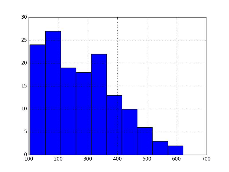
Histogram of Airline Passengers
Reviewing the plot of the time series again, we can see that there is an obvious seasonality component, and it looks like the seasonality component is growing.
This may suggest an exponential growth from season to season. A log transform can be used to flatten out exponential change back to a linear relationship.
Below is the same histogram with a log transform of the time series.
|
1 2 3 4 5 6 7 8 9 10 |
from pandas import read_csv from matplotlib import pyplot from numpy import log series = read_csv('international-airline-passengers.csv', header=0, index_col=0) X = series.values X = log(X) pyplot.hist(X) pyplot.show() pyplot.plot(X) pyplot.show() |
Running the example, we can see the more familiar Gaussian-like or Uniform-like distribution of values.
Histogram Log of Airline Passengers
We also create a line plot of the log transformed data and can see the exponential growth seems diminished, but we still have a trend and seasonal elements.
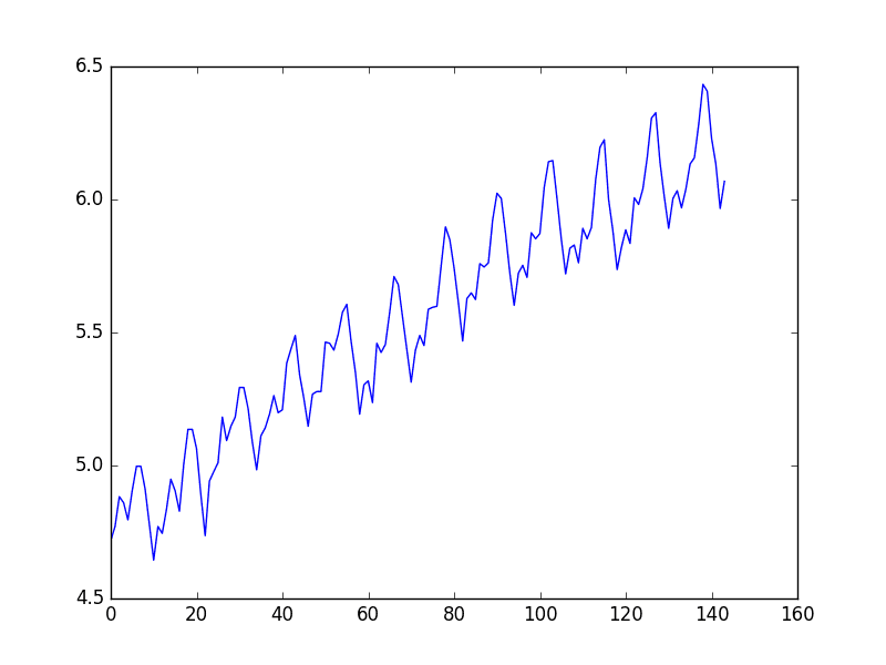
Line Plot Log of Airline Passengers
We can now calculate the mean and standard deviation of the values of the log transformed dataset.
|
1 2 3 4 5 6 7 8 9 10 11 12 |
from pandas import read_csv from matplotlib import pyplot from numpy import log series = read_csv('international-airline-passengers.csv', header=0, index_col=0) X = series.values X = log(X) split = round(len(X) / 2) X1, X2 = X[0:split], X[split:] mean1, mean2 = X1.mean(), X2.mean() var1, var2 = X1.var(), X2.var() print('mean1=%f, mean2=%f' % (mean1, mean2)) print('variance1=%f, variance2=%f' % (var1, var2)) |
Running the examples shows mean and standard deviation values for each group that are again similar, but not identical.
Perhaps, from these numbers alone, we would say the time series is stationary, but we strongly believe this to not be the case from reviewing the line plot.
|
1 2 |
mean1=5.175146, mean2=5.909206 variance1=0.068375, variance2=0.049264 |
This is a quick and dirty method that may be easily fooled.
We can use a statistical test to check if the difference between two samples of Gaussian random variables is real or a statistical fluke. We could explore statistical significance tests, like the Student t-test, but things get tricky because of the serial correlation between values.
In the next section, we will use a statistical test designed to explicitly comment on whether a univariate time series is stationary.
Augmented Dickey-Fuller test
Statistical tests make strong assumptions about your data. They can only be used to inform the degree to which a null hypothesis can be rejected or fail to be reject. The result must be interpreted for a given problem to be meaningful.
Nevertheless, they can provide a quick check and confirmatory evidence that your time series is stationary or non-stationary.
The Augmented Dickey-Fuller test is a type of statistical test called a unit root test.
The intuition behind a unit root test is that it determines how strongly a time series is defined by a trend.
There are a number of unit root tests and the Augmented Dickey-Fuller may be one of the more widely used. It uses an autoregressive model and optimizes an information criterion across multiple different lag values.
The null hypothesis of the test is that the time series can be represented by a unit root, that it is not stationary (has some time-dependent structure). The alternate hypothesis (rejecting the null hypothesis) is that the time series is stationary.
- Null Hypothesis (H0): If failed to be rejected, it suggests the time series has a unit root, meaning it is non-stationary. It has some time dependent structure.
- Alternate Hypothesis (H1): The null hypothesis is rejected; it suggests the time series does not have a unit root, meaning it is stationary. It does not have time-dependent structure.
We interpret this result using the p-value from the test. A p-value below a threshold (such as 5% or 1%) suggests we reject the null hypothesis (stationary), otherwise a p-value above the threshold suggests we fail to reject the null hypothesis (non-stationary).
- p-value > 0.05: Fail to reject the null hypothesis (H0), the data has a unit root and is non-stationary.
- p-value <= 0.05: Reject the null hypothesis (H0), the data does not have a unit root and is stationary.
Below is an example of calculating the Augmented Dickey-Fuller test on the Daily Female Births dataset. The statsmodels library provides the adfuller() function that implements the test.
|
1 2 3 4 5 6 7 8 9 10 |
from pandas import read_csv from statsmodels.tsa.stattools import adfuller series = read_csv('daily-total-female-births.csv', header=0, index_col=0, squeeze=True) X = series.values result = adfuller(X) print('ADF Statistic: %f' % result[0]) print('p-value: %f' % result[1]) print('Critical Values:') for key, value in result[4].items(): print('\t%s: %.3f' % (key, value)) |
Running the example prints the test statistic value of -4. The more negative this statistic, the more likely we are to reject the null hypothesis (we have a stationary dataset).
As part of the output, we get a look-up table to help determine the ADF statistic. We can see that our statistic value of -4 is less than the value of -3.449 at 1%.
This suggests that we can reject the null hypothesis with a significance level of less than 1% (i.e. a low probability that the result is a statistical fluke).
Rejecting the null hypothesis means that the process has no unit root, and in turn that the time series is stationary or does not have time-dependent structure.
|
1 2 3 4 5 6 |
ADF Statistic: -4.808291 p-value: 0.000052 Critical Values: 5%: -2.870 1%: -3.449 10%: -2.571 |
We can perform the same test on the Airline Passenger dataset.
|
1 2 3 4 5 6 7 8 9 10 |
from pandas import read_csv from statsmodels.tsa.stattools import adfuller series = read_csv('international-airline-passengers.csv', header=0, index_col=0, squeeze=True) X = series.values result = adfuller(X) print('ADF Statistic: %f' % result[0]) print('p-value: %f' % result[1]) print('Critical Values:') for key, value in result[4].items(): print('\t%s: %.3f' % (key, value)) |
Running the example gives a different picture than the above. The test statistic is positive, meaning we are much less likely to reject the null hypothesis (it looks non-stationary).
Comparing the test statistic to the critical values, it looks like we would have to fail to reject the null hypothesis that the time series is non-stationary and does have time-dependent structure.
|
1 2 3 4 5 6 |
ADF Statistic: 0.815369 p-value: 0.991880 Critical Values: 5%: -2.884 1%: -3.482 10%: -2.579 |
Let’s log transform the dataset again to make the distribution of values more linear and better meet the expectations of this statistical test.
|
1 2 3 4 5 6 7 8 9 10 11 |
from pandas import read_csv from statsmodels.tsa.stattools import adfuller from numpy import log series = read_csv('international-airline-passengers.csv', header=0, index_col=0, squeeze=True) X = series.values X = log(X) result = adfuller(X) print('ADF Statistic: %f' % result[0]) print('p-value: %f' % result[1]) for key, value in result[4].items(): print('\t%s: %.3f' % (key, value)) |
Running the example shows a negative value for the test statistic.
We can see that the value is larger than the critical values, again, meaning that we can fail to reject the null hypothesis and in turn that the time series is non-stationary.
|
1 2 3 4 5 |
ADF Statistic: -1.717017 p-value: 0.422367 5%: -2.884 1%: -3.482 10%: -2.579 |
Summary
In this tutorial, you discovered how to check if your time series is stationary with Python.
Specifically, you learned:
- The importance of time series data being stationary for use with statistical modeling methods and even some modern machine learning methods.
- How to use line plots and basic summary statistics to check if a time series is stationary.
- How to calculate and interpret statistical significance tests to check if a time series is stationary.
Do you have any questions about stationary and non-stationary time series, or about this post?
Ask your questions in the comments below and I will do my best to answer.
Want to Develop Time Series Forecasts with Python?

Develop Your Own Forecasts in Minutes
...with just a few lines of python codeDiscover how in my new Ebook:
Introduction to Time Series Forecasting With Python
It covers self-study tutorials and end-to-end projects on topics like: Loading data, visualization, modeling, algorithm tuning, and much more...
Finally Bring Time Series Forecasting to
Your Own Projects
Skip the Academics. Just Results.


")


Hi there, nice post!
Just a quick question, when testing the residuals of an OLS regression between two price SERIES for stationarity would you consider then, the two price series, to be cointegrated If the H0 was rejected by the ADF test that you ran on the residuals ?
Or would you first run the ADF test on each of the price series in order to see if they are I(1) themselves?
Thanks!
Hi Eduardo,
Both. I would check both the input data and the residuals.
Can you help with material .for this project topic. Comparison of different method of stationalizing time series data. You can inbox me on this mail box. adedayo.temmy@yahoo.com. thanks
Hi Jason,
Thanks for the reply!
I asked this because of a “common sense” (maybe not) assumption that price series would not be, per se, stationary, by definition, so, sometimes I ask myself if isn’t this kind of testing a little too much.
Best Regards!
I’m high on ML methods for time series over linear methods like ARIMA, but one really important consideration is stationarity.
Trend removal and exploring seasonality specifically is a big deal otherwise ML methods blow-up for the same reasons as linear methods.
I’d like to do a whole series of posts on stationarity.
Hi . What kind of methods are well for removing checking time series is :
1. trendy
2. stationary
3. has seasonality
I would like to forcats time series via RNN, but for getting more accuarate results I need at the beging check all this 3 characteristics.
Data visualization is a good start.
beside using log, do you consider to use panda.diff()?
Thanks Cipher, it beats doing the difference manually.
Hi Jason,
I am not sure I understand why in the case of the airline dataset you also checked the log. Because the first test shows that the data is not stationary. Why would you do the test on the logs as well? In other words, let’s say the adfuller test on the log showed that the log of this dataset is stationary; It still doesn’t change the fact that the dataset itself is non-stationary.
A power transform like a log can remove the non-stationary variance – as we see in this dataset.
I think what he means is that when you do power transform (log) to a non-stationary variance, and do testing on it (adf) and build a model also. That only applies to the transformed data. But how about the original , non-transformed dataset?
We no longer work with the raw data, we work on the transformed data. We continue to apply transforms until we get something stationary, then fit a model.
Does that help?
great article! easy to understand. simplicity is powerful. and all those good stuff.
Thanks Seine. I’m glad you found it useful.
“We interpret this result using the p-value from the test. A p-value below a threshold (such as 5% or 1%) suggests we accept the null hypothesis (non-stationary), otherwise it suggests we reject the null hypothesis (stationary)”
Shouldn’t this be the opposite of what you have stated. Please see http://stats.stackexchange.com/questions/55805/how-do-you-interpret-results-from-unit-root-tests
Hi Jack,
Yes, that is a typo, fixing now and I made it clearer with some more bullet points. All of the analysis in the post is correct.
In summary, the null hypothesis (H0) is that there is a unit root (autoregression is non-stationary). Rejecting it means no unit root and non-stationary.
A p-value more than the critical value means we cannot reject H0, we accept that there is a unit root and that the data is non-stationary.
Hi Jason, thank you for the great article, but i think but you fixed the typo in the opposite way, if i’m not mistaken it’s more like ” We interpret this result using the p-value from the test. A p-value below a threshold (such as 5% or 1%) suggests we accept the null hypothesis (stationary), otherwise it suggests we reject the null hypothesis (non-stationary) “
My bad it’s correct, I confused it with the H0 of stationar tests
No problem. It is confusing.
Autoregression need not to be non-stationary. Take AR(1) e.g.
I performed the Augmented Dickey-Fuller test on my own data set. My result are as follows:
ADF Statistic: -34.360229
p-value: 0.000000
Critical Values:
1%: -3.430
5%: -2.862
10%: -2.567
So my time series are stationary. In my example, I have 525600 values giving me a maxlag of 102. These are minute data for one month. But I don’t understand how so few lags can detect e.g a daily variation?
Now when I calculate the distribution of occurrence frequency, there is clearly a time dependence on UT on hourly binned data. I have a higher number of samples, for a certain range of values, at around 15 UT compared to other times. So I have a UT dependence in my data, but it is still stationary. So I guess one should be careful when using this test. In my case there is a UT dependency on the number of values, at a certain level, rather than the value itself. How to deal with this? One idea, perhaps, is to add sine and cosine of time to the inputs. Any comments on this?
Interesting. Perhaps it would be worth performing a stationary test at different time scales?
Yes, I did. Same result. I also performed the test on the sunspot number, from one of your earlier posts. I then got this result:
ADF Statistic: -9.567668
p-value: 0.000000
Critical Values:
1%: -3.433
5%: -2.863
10%: -2.567
Now, I am really confused. I also did a test on artificial data from a sine function with normally distributed data added to it. Now the test gave a p-value of 0.07, but from the plot it was very obvious the data is non-stationary. So I really suggest to use the group by process in Pandas and plot the data.
Another approach, instead of removing seasonality is the following. If only the target values, used for training a prediction model, are non-stationary, then it might be easier to add sine/cosine of time to the inputs. Of course, the input space increases but there is no need to create time-lagged data for these inputs.
I appreciate any comments and suggestions.
I’m dubious about your results.
I have found the test to be reliable.
Perhaps the version of the statsmodels library is out of date, or perhaps the data you have loaded does not match your expectation?
The problem is the way you are printing out the results. Can you just print the whole variable like this
print(result)
or something like this
print(‘ADF Statistic: {}’.format(result[0])).
I was having the same problem, but changing the printing format, fixed it for me.
ADF Statistic: -12.851066
p-value: 0.000000
Critical Values:
1%: -3.431
5%: -2.862
10%: -2.567
Results of Dickey-Fuller Test:
Test Statistic -1.152597e+01
p-value 3.935525e-21
#Lags Used 2.300000e+01
Number of Observations Used 1.417000e+03
Critical Value (5%) -2.863582e+00
Critical Value (1%) -3.434973e+00
Critical Value (10%) -2.567857e+00
dtype: float64
Hi , I want to forecast temperature of my time series dataset. Dickey -Fuller test in python gives me above results, which shows Test statistics is larger than any of the critical value meaning time series is not stationary after taking transformations. So ,can i forecast without time series being non-stationary?
You can, but consider another round of differencing.
What code did you use to get this, Joy? I’m trying to get results like that but I only get the graph
Does the statsmodel python library require us to convert the series into stationary series before feeding the series to any of the ARMA or ARIMA models ?
Ideally, I would. The model can difference to address trends, but I would recommend explicitly pre-processing the data before hand. This will help you better understand your problem/data.
Great article, you make these topics understandable.
I started testing some series for stationarity and got strange behaviors I cannot understand.
In Python (3.6), ADF give so different results for linear sequences of 100 and 101 items:
from statsmodels.tsa.stattools import adfuller
adfuller(range(100))
adfuller(range(101))
give ADF statistics of +2.59 and -4.23.
I’d expect both results to be very close to each other. Neither is stationary series is stationary as the express the same trend. But the test is positive in one case and negative in the other.
What is wrong?
I would not worry, focus on the test (e.g. the value relative to critical value), not the value itself.
Thanks for the quick reply.
But this is precisely my problem: with a slight change in the number of observations of a series of constant slope/trend of +1, the test swings entirely from non-stationary to stationary for a reason I fail to understand.
from statsmodels.tsa.stattools import adfuller
X=range(100)
result = adfuller(X)
print(‘ADF Statistic: %f’ % result[0])
print(‘p-value: %f’ % result[1])
for key, value in result[4].items():
print(‘\t%s: %.3f’ % (key, value))
ADF Statistic: 2.589283
p-value: 0.999073
1%: -3.505
5%: -2.894
10%: -2.584
X=range(101)
result = adfuller(X)
print(‘ADF Statistic: %f’ % result[0])
print(‘p-value: %f’ % result[1])
for key, value in result[4].items():
print(‘\t%s: %.3f’ % (key, value))
ADF Statistic: -4.232578
p-value: 0.000580
1%: -3.504
5%: -2.894
10%: -2.584
Ah I see. It might be a case of requiring a critically minimum amount of data for the statistical test to be viable.
Thanks for sharing the knowledge!
quick questions if you don’t mind: I would like to test a few trading strategies on ETFs. It looks obvious that these time series are non stationary.
how does one go about converting them to stationary?
I would like to use Technical Indicators (which input are prices) as features in my model. What shall I do to the features?
my objective is not to predict price but to classify into “buy/sell” (or hold).
any algo better suited for financial time series?
Thank you!
You can use differencing and seasonal adjustment. I have posts on both methods, use the search feature.
Actually, when ADF Statistic < critical value then it is stationary. Comparing pvalue with critical value is not right and confusing. Including the adfuller api explanation in http://www.statsmodels.org/dev/generated/statsmodels.tsa.stattools.adfuller.html.
I don’t think we are comparing the p-value to anything in this post, I believe are reviewing the test statistic.
I see. It is ADF Statistic < critical value or p-value < threshold, then the series is stationary. Threshold is 0.05 etc.
Perhaps I’m dense, but where exactly? Can you quote the text?
I note that I describe how to interpret p-values separately from interpreting test static.
From your blog.
p-value <= 0.05: Reject the null hypothesis (H0), the data does not have a unit root and is stationary.
And there is another explanation based on critical value.
https://www.analyticsvidhya.com/blog/2016/02/time-series-forecasting-codes-python/
So there are two ways of considering the adf result, using p-value or using critical value.
In that section, I was introducing the meaning of the p-value, not how to interpret the test. Sorry for the confusion.
I performed the Dickey–Fuller test and get 1 as p-value. Then I performed Box_Cox transform which allowed to decrease p-value to 0.96. Then I performed seasonal differentiation and p-value decreased to 0.0000. After this, I build LSTM neural network and train it. Now, I want to compare results in the original scale, in the transformed. I found the scipy.special.inv_boxcox() function, which does the inverse transformation. But for me, it is not working. What can be wrong?
Perhaps you can experiment on some test data separate from your model. Transform and then inverse transform.
Remember all operations need to be reversed, including the seasonal adjustment.
Excellent!
Thanks.
I’m very interested in your articles Jason, I have a question.
If I train my model using the residual data ( removing seasonal and trends), what about the predicted values how we get the correct values ( how to add seasonally and trends again) .
I hope that I can present my question correctly. sorry for my poor English.
additional remark,
Why you don’t use the package “statsmodels” to decompose the time series. I mean the issue discussed here:
https://stackoverflow.com/questions/20672236/time-series-decomposition-function-in-python
If you remove the trend and seasonality prior to modeling, you can add them back to the prediction.
If you used differencing, invert the differencing. If you used a model, invert the application of the model.
I have many examples on the blog of this.
HI Jason,
I am looking for he blog posts noted above regarding how to re-add trends and seasonality to modeling after it has been removed. Could you please point me to the blog posts which cover this? I cannot seem to locate them.
Thanks much,
Joe
If you remove the trend by differencing or the seasonality by seasonal differencing, you can add it back directly, via addition with the value that was subtracted.
Perhaps this will help:
https://machinelearningmastery.com/machine-learning-data-transforms-for-time-series-forecasting/
Hi Jason, as far as I know adfuller is a statistical test for Random walk, H1 means not Random walk, above you revealing that H1 also means stastionary time-series, does any non-random walk is stationary?
The test checks for a unit root:
https://en.wikipedia.org/wiki/Augmented_Dickey%E2%80%93Fuller_test
A random walk is not stationary.
I think it is worth mentioning that to apply the ADF test, we assume that the time series follows a given model (dy(t)=cst+gamma*y(t-1)+….+e(t)) where e(t) is the error term that is supposed to be a white noise.
So if you reject H0, and that indeed the error term is white noise and that gamma<1 then the model will be stationary (I think in the strict sense – cf https://people.maths.bris.ac.uk/~magpn/Research/LSTS/TOS.html for the different definitions of stationarity)
Thanks for the note.
Traceback (most recent call last):
File “shampoo.py”, line 20, in
result = adfuller(X)
File “/home/denis/.local/lib/python3.5/site-packages/statsmodels/tsa/stattools.py”, line 221, in adfuller
xdall = lagmat(xdiff[:, None], maxlag, trim=’both’, original=’in’)
File “/home/denis/.local/lib/python3.5/site-packages/statsmodels/tsa/tsatools.py”, line 397, in lagmat
nobs, nvar = xa.shape
ValueError: too many values to unpack (expected 2)
I have some suggestions here:
https://machinelearningmastery.com/faq/single-faq/why-does-the-code-in-the-tutorial-not-work-for-me
Hi Jason,
Nice tutorial! I’m just starting out with time series data so I’m wondering, if my data doesn’t pass stationarity tests, then I cannot use time series analysis on it, is that right? Can RNNs model time series that are non-stationary?
You can, but results might not be good.
RNNs do seem to perform better with a stationary series in my experience.
Hi,
I guess trend-stationary series is the one that has a trend but no unit root. Correct me if I am wrong .
Reference : http://in.mathworks.com/help/econ/trend-stationary-vs-difference-stationary.html
Hi Jason,
I have a small question, when you are working with ADF when the result suggests stationary is it difference stationary, stationary in increments or normal weak stationary in time series…….
The statistical test is reporting a likelihood of being stationary rather than a fact.
I am working with a time series that has multiple random measurements for every moment in time. In other words, my X series includes sets of distinct measured values for every timestamp.
Will the described procedure and code work for me as is? Should I be sorting such X or not?
You would need to work with each time series (variable) separately.
Thank you for your explanations!It is quite interesting
After the evaluation of the model, how can we visualize the predicted data to complete the available database
thanks
Thanks. You can use the matplotlib plot() function to plot yhat vs y
Hi Jason. In the example above you used ADF to test whether the Gaussian normally distributed sample is stationary. 1) Any hints on what to do if we try to model a process that shows a non-Gaussian distribution? 2) Can we still make inferences about stationarity based on means/variances of two subsamples from a non-Gaussian process? 3) Could you please point me to a reference with a nice description of how to test for stationarity in non-normal samples and how to model such time series? Thanks!
Good question, using a data visualization is always a great fall-back.
I need codes for Bai Perron test,KPSS test and Phillips Perron test
Perhaps try a google search?
Hi, this is a very interesting tutorial. Thanks a lot.
I am having about 1000+ different time-series dataset in the format of (year,number) and need to forecast the values for each and every dataset in next 5 years.As i have lot of datasets, I would like to know if there is a way to automate the aforementioned stationary check step, so that I can directly perform the ARIMA process? or is there any other algorithm that you would recommend?
Perhaps difference all datasets before modeling?
Thanks a lot for the suggestion. Did you mean performing ‘log’ as ‘difference’? And after that using the p-value of Augmented Dickey-Fuller test to decide the stationary?
Just curious to know, does performing ‘log’ guarantee that you have a stationary time-series dataset?
Log and other power transforms can calm an increasing/changing variance and make the data distribution more Gaussian.
Log transform does not work,and how can we do the next for this situation?
Thanks.
What do you mean it does not work?
The turth is that the time series is still non-stationary.How can we get the stationary time series ?
You can remove the trend by differencing, you can remove the seasonality by seasonal differencing.
I have posts on both topics, perhaps start here:
https://machinelearningmastery.com/start-here/#timeseries
Thanks Jason, great article.
However could you please advice how would you approach stationarity test with multivariate, multiinput and multioutput time series?
I’m working on multistep prediction for a few thousands of different elements. For each element, i’ll probably have to use a few different kind of measurements (like temperature, pressure, traffic etc.). I have to predict three timeseries for each site. For some network elements measurements goes up, for others they go down… How should i approach stationarity test properely in that case? Should i check and transform for each element separately? Or perform the stationarity test for each aggregated by time measurement (over the whole set of elements)? What do you suggest?
Regards.
I would start by performing a test on each separate univariate series.
Then test if making one or all series stationary impacts model performance, e.g a linear model.
Thanks Jason!
I have a question related to the Augmented Dickey-Fuller (ADF) test that you applied with the “International airline passengers” dataset. When ADF test is applied using R we get different decision results than when using python. Here are the numbers.
Using R:
library(tseries)
tsData <- AirPassengers # ts data
adf.test(as.timeseries(tsData)) # p-value < 0.05 indicates the TS is stationary
Out:
Augmented Dickey-Fuller Test
data: tsData
Dickey-Fuller = -7.3186, Lag order = 5, p-value = 0.01
alternative hypothesis: stationary
Warning message:
In adf.test(tsData) : p-value smaller than printed p-value
Conclusion: Reject Ho. So we accept it is stationary.
Using Python:
from pandas import Series
from statsmodels.tsa.stattools import adfuller
series = Series.from_csv('daily-total-female-births.csv', header=0)
X = series.values
result = adfuller(X)
print('ADF Statistic: %f' % result[0])
print('p-value: %f' % result[1])
print('Critical Values:')
for key, value in result[4].items():
print('\t%s: %.3f' % (key, value))
Out:
ADF Statistic: 0.815369
p-value: 0.991880
Critical Values:
5%: -2.884
1%: -3.482
10%: -2.579
Conclusion: No Reject Ho. So we no accept it is stationary. Then it looks Non-stationary
The test statistic is positive, meaning we are much less likely to reject the null hypothesis (it looks non-stationary).
Both datasets (R: AirPassengers and Python: daily-total-female-births) are the same. So, I can not get the reasons why ADF test showed different results.
Would you please give me a hand in finding an explanation of this rare situation?
The airline dataset is not stationary. If a library reports that it is, perhaps there is a bug in your code or the library?
The right R code is:
library(tseries)
tsData <- AirPassengers # ts data
adf.test(tsData)
AirPassengers
Out:
Jan Feb Mar Apr May Jun Jul Aug Sep Oct Nov Dec
1949 112 118 132 129 121 135 148 148 136 119 104 118
1950 115 126 141 135 125 149 170 170 158 133 114 140
1951 145 150 178 163 172 178 199 199 184 162 146 166
1952 171 180 193 181 183 218 230 242 209 191 172 194
1953 196 196 236 235 229 243 264 272 237 211 180 201
1954 204 188 235 227 234 264 302 293 259 229 203 229
1955 242 233 267 269 270 315 364 347 312 274 237 278
1956 284 277 317 313 318 374 413 405 355 306 271 306
1957 315 301 356 348 355 422 465 467 404 347 305 336
1958 340 318 362 348 363 435 491 505 404 359 310 337
1959 360 342 406 396 420 472 548 559 463 407 362 405
1960 417 391 419 461 472 535 622 606 508 461 390 432
class(AirPassengers)
Out:
[1] "ts"
frequency(AirPassengers)
Out:
[1] 12
I run the test again but now using your dataset as a source (converting it to” ts” class in R) and I got the same result.
Anyway, there is something definitely wrong in this way to present the stationarity study of this dataset by using the Augmented Dickey-Fuller (ADF) test in R.
There are many articles on the web (www) that using just the ADF test with R conclude that the AirPassengers dataset is stationary when clearly is not.
I agree with you 100%. I mean, considering R if we complement our study using other test and Autocorrelation analysis we can get the same conclusion that the AirPassengers dataset is not a stationary one.
Thanks for your answer and time, of course.
Regards.
HA
Interesting. Perhaps there is a bug in the routine, or a change in the way the test must be interpreted in R? I think the latter is more likely.
Hi,
I have a question about time series modeling. I implemented a multilinear regression in Python, but I found on Eviews that a threshold regression would be better.
Do you know how to implement this new model with Python ? I didn’t find the solution for the moment.
Thank you very much for your answer.
Alex
I’m not familiar with that algorithm, perhaps ask the author?
Hi Jason,
Great post! I am new to time series analysis. I have questions for you, is that a high autocorrelation plot (even lags = 100) means the time series is non-stationary? Since I used all methods of yours, and it seems the data should be stationary, but after plot the autocorrelation, It still gives me a high result.
Not necessarily, if you calculate the ACF/PACF after removing trends and seasonality, it could be stationary and still have high correlation (I think – off hand).
Thanks so much prof..
ive been trying to reach you sir ..
my test was -2 for adf and didnt pass any of the significance test,
do you think phillip perron test is a good idea ?
I am not familiar with that test, sorry.
Hi Jason,
Great content!
If after applying ADF test on my time series, I get NULL hypothesis true, then that means that the time series follows a random walk process.
Which means that trying to make the series stationary wouldn’t work right? Because random walk means no learnable pattern.
Differencing the series will give me a trend stationary time series but non stationary variance.
Am I correct? Or is there some transformation that could work?
A random walk is non-stationary, but not all non-stationary time series are a random walk.
Try differencing to make it stationary.
But isn’t ADF testing for the presence of a unit root? And presence of unit root implies a random walk. This is my understanding. That is where the confusion is: if the ADF null hypothesis is accepted, then forecasting shouldn’t work.
That is not my understanding.
Unit root means non-stationary, probably trend non-stationary:
https://en.wikipedia.org/wiki/Dickey%E2%80%93Fuller_test
Okay. My bad!
So Random Walk is specifically for the case when coefficient of Y(t-1) term is 1 and the process is AR(1) ?
Xt = b0 + b1×X(t-1) + εt
i.e. random walk is a special case of AR(1) process where b1 = 1.
Correct this time, right?
Sure, more here:
https://machinelearningmastery.com/gentle-introduction-random-walk-times-series-forecasting-python/
Hi!
thanks for the great content!
I have a question I’ll appreciate if you could help me!
is it possible that we see an OBVIOUS trend in the plot, but still get the result that the TS is stationary form the Dickey-Fuller test?
Probably not.
I have a small question, how can I cite the material you have presented here
Sorry, Mainly the reference for the ADF test case
I show how here:
https://machinelearningmastery.com/faq/single-faq/how-do-i-reference-or-cite-a-book-or-blog-post
Hi Jason:
Do you have any article on VAR and VARMAX using statsmodels module of Python?
Any idea on how to measure the error of forecasting for those models in terms of MAE?
Thanks
I don’t have a tutorial on VAR or VARMAX.
Yes, you can use sklearn to calculate MAE:
https://scikit-learn.org/stable/modules/classes.html#sklearn-metrics-metrics
Hi Jason,
Do you have any article on checking stationarity for multivariate time series forecasting methods?
It would be great you can share VAR module using Python as well.
Thanks,
Aman
I do not, only univariate data.
Thanks for the suggestion.
Hi Jason, Hw r u?
How I can handle a log plot if a have some zero in my time-series? My target is predict rain. Is not stationary. I got a error follow this approach: divide by zero encountered in log.
thanks.
You can create a log plot by adding a value to all samples to ensure all values are positive.
Hello Jason,
ADF Statistic: -4.808291
p-value: 0.000052
Critical Values:
5%: -2.870
1%: -3.449
10%: -2.571
Here since -4 for ADF statistic is less than all critical values means we reject the null hypothesis, but p-value 0.000052 is greater than 5% (-2.870) so we fail to reject null hypothesis ? How should we know ?
I mean we are getting conflicting results ?
No.
p-value <= 0.05 means we reject. -4.808291 <= -3.449 means we reject. Reject in both cases.
Sorry Jason, I forgot that p-value must be less than 0.05 rather than the critical value at 5%. It was after I asked I found the mistake XD
No problem at all, it can get confusing.
Hi Jason,
A clarification on this statement please – “The intuition behind a unit root test is that it determines how strongly a time series is defined by a {trend}.”
I came across an example time series which is “Trend Stationary” but clearly is seasonal. ADF is reporting a VERY low p-value for it.
So, I am wondering,
1. If stationary means absence of both trend and seasonality, is there a different test to check for complete stationarity (tread and seasonal)?
2. Or can the models work well as long as time series is trend stationary?
Please advise. Many thanks.
Yes, it won’t be stationary if there is seasonality. Often it is simpler to just talk about trends, but you’re right.
A stationary time series has neither a trend nor seasonality.
Hi Jason,
as in statsmodel’s docs:
statsmodels.tsa.stattools.adfuller(x, maxlag=None, regression=’c’, autolag=’AIC’, store=False, regresults=False)
if we use the default values, maxlag will be 12*(nobs/100)^{1/4} by default, and the number of lags is chosen to minimize the corresponding information criterion (in this case AIC)
My question is:
if the returned lag, result[2], is 14, do you have an idea if we must take all lags up to 14 or just the 14th lag ?
Many thanks in advance
All lags up to 14th by default.
To be more selective about lags in that interval, a custom model may be required.
Hi Jason,
I’m looking at the VXO and some other stock market data.
For the VXO seasonal decompose shows some trend and strong seasonality, but AD-Test suggests the data is stationary. I didn’t perform any kind of transformation here.
For the S&P500 on the other hand side i had to use log returns to achieve stationarity. Is this possible? I’m struggling to understand the difference.
In case this is perfectly fine: can i use both series as input for the same model like that (let’s say OLS to begin with), or do they have to get the same treatment i.e. the same transformation to lead to useful results?
Thank you very much in advance for your reply.
Different time series may have to be made stationary in different ways. Once stationary, they can be modelled.
Doc Jason strikes again! This post gave me tremendously good insight! Almost done with my use case but a good colleague at work throws at me the most important test for my (magnitude, time) paired data – how do you test for the presence of seasonality if stationary? Augmented Dickey-Fuller test is. Thanks again.
Happy that it helped!
If you have seasonality, the data is not stationary.
Hi,
I am getting below results for Dickey-Fuller Test. Can someone suggest technique to make my data stationary.
I could see that graph pattern for actual data, rolling mean, rolling std is also almost same.
I have already tried log transformation, differencing and the results are still same 🙁
Results of Dickey-Fuller Test:
Test Statistic -8.161630e+00
p-value 9.110753e-13
#Lags Used 2.000000e+01
Number of Observations Used 1.351000e+03
Critical Value (1%) -3.435200e+00
Critical Value (5%) -2.863682e+00
Critical Value (10%) -2.567910e+00
dtype: float64
Regards,
Sai
Perhaps try differencing the trend and the seasonality separately – if both exist?
https://machinelearningmastery.com/remove-trends-seasonality-difference-transform-python/
Also try box-cox power transform?
Nice tutorial! I just have a question. I have a date series with high variance and as a solution do the transform log on it. The thing is it changed the data on my date series, and when I do forecasting, it only forecast according to that changed/transform data ( although it greatly improves my model with a MSE of 1+ something only compare to 500+ something before).How can I bring it back where I can actually forecast the real values (but using the model from the transformed date series) or what approach is needed on this kind of scenario….
I don’t understand, sorry.
You fit a model on historical data, then use the model to make predictions on the future. Sometimes we prepare the historical data prior to fitting the model.
Which part are you having trouble with exactly?
If you need help making a prediction, e.g. calling predict(), this might help:
https://machinelearningmastery.com/make-sample-forecasts-arima-python/
Hi Jason,
Thanks for this post, it is very helpful. I did the Dickey-Fuller test on my data and I got a zero p-value.
What does it mean? I read that it might mean that probably the data does not have normal distribution and are not stationary. Could it be the case? Below are the results of the test:
Test statistic = -4.539
P-value = 0.000
Critical values :
1%: -3.453342167806272
5%: -2.871663828287282
10%: -2.572164381381345
It may suggest the data is stationary.
Perhaps plot to confirm.
Great tutorial, just one more question. What if in the end you find out that the time series data is non-stationary. Do you continue building model from it? Or do you find another time series data that can be build upon better.
Thanks.
You can make it stationary using differencing, seasonal differencing and power transforms.
Hi Jason.
I have a doubt how to prepare this dataset (link below). Can you give a suggestion please?
It appears a non-stacionary series, correct?
Original dataset plot:
https://pasteboard.co/IEdYWWx.png
I tried to apply the diference method with 365 days
diff = difference(values, 365)
Dataset plot after difference:
https://pasteboard.co/IEe4rko.png
The procedure is that?
Thanks.
Yes, looks like seasonality.
Perhaps you need to perform seasonal differencing twice?
Hi Jason.
I have to evaluate the RMSE with normalized or non-normalized data?
The result of RMSE are the same for the both ?
Thanks.
Typically you evaluate error on data with all transforms reversed so the units are the same as the original data.
Good post, Jason and thanks!
I was wondering (assuming we had no prior knowledge) which X or Y was the independent variable and vice versa.. is there a way to determine one or the other?
Perhaps you’re referring to correlation? E.g.:
https://machinelearningmastery.com/how-to-use-correlation-to-understand-the-relationship-between-variables/
Hi Jason ,
Thank you for your email and for every things. I still learn from you and your book.
Please just I have two questions regarding the How to Check if Time Series Data is Stationary with Python.
My original data has trend that from the test of mean and variance values and by the visual observation it has trend.
and you know that to remove the trend I need to apply the first differencing or second differencing.
Please, Is applying the differencing method to remove the trend will affect my original data values?
Please, Is there any other method to remove the trend instead of differencing method?
Thank you.
Regards,
Yes, differencing will change your original data, this is the goal.
Yes, you can fit a linear model and subtract it from the data.
Hi, I was trying to run the same code as you have shown in this article, it seems that passing:
from statsmodels.tsa.stattools import adfuller
series = read_csv(‘daily-total-female-births.csv’, header=0, index_col=0)
X = series.values
result = adfuller(X)
Shows the following error:
ValueError: too many values to unpack (expected 2)
I fixed this issue by using the following code:
import statsmodels.tsa.stattools as tsa
series = read_csv(‘daily-total-female-births.csv’, header=0, index_col=0)
result = tsa.adfuller(series[‘Births’])
I am very confused as to what the difference between the two code blocks shown above is.
Excellent site and keep up the good work.
John
One more small bug I found in the code:
split = (len(X) / 2) ### this returns 182.5 for female births csv
X1, X2 = X[0:split], X[split:]
The slicing procedure is expecting an integer for X1 & X2 so it returns an error if len(X) is an odd number,
I fixed this by using the following code:
split = round(len(X)/2)
Nice, thanks!
I have updated the examples.
Looks like a bug in the loading of the dataset. I must have introduced it in the update.
Thanks! Fixed.
Hello Jason, thanks for all the tutorials! I performed the ADF test on my time series data and it gave me the following results . DO you read this as it means its stationary and i can just go for the time series algorithm ? thanks!
Results of Dickey-Fuller Test:
Test Statistic -6.817677e+00
p-value 2.039396e-09
#Lags Used 6.000000e+00
Number of Observations Used 7.770000e+02
Critical Value (1%) -3.438794e+00
Critical Value (5%) -2.865267e+00
Critical Value (10%) -2.568755e+00
dtype: float64
It looks stationary.
thanks! if i try to log the data it keeps telling that it encountered divided by zero in log . any suggestions how to deal with that other than not use the log of the data? thanks!
Make the data positive before using the log transform.
Hi Jason,
I ran the adfuller and output is as below:
ADF Statistic: -2.457146p-value: 0.126252Critical Values: 1%: -3.438, 5%: -2.865, 10%: -2.569https://github.com/RSwarnkar/temporary/blob/master/timeseries2.png
Is series stationary or non-stationary?
regards,
Rajesh
Not stationary.
Do you plan to have a login feature into website so that I can check my past comments and replies?
Thanks !
And a separate discussion domain would be awesome too !
Good suggestion.
Not at this stage.
Hello Jason
A missing casting in line 4 should be added for Python version 3.7.
from pandas import read_csv
series = read_csv(‘international-airline-passengers.csv’, header=0, index_col=0)
X = series.values
split = int(len(X) / 2)
X1 = X[0:split]
X2 = X[split:]
mean1, mean2 = X1.mean(), X2.mean()
var1, var2 = X1.var(), X2.var()
print(‘mean1=%f, mean2=%f’ % (mean1, mean2))
print(‘variance1=%f, variance2=%f’ % (var1, var2))
The rest code samples are ok
E. Bonilla
Great suggestion, thanks!
following is the output of my adfuller() func.
I understand this means my time series is stationary ? is there any other interpretations that can be derived form this?
Can i fit this into an ARIMA model to predict future values?
ADF Statistic: -4.453993
p-value: 0.000238
Critical Values:
1%: -3.433
5%: -2.863
10%: -2.567
Yes, stationary.
I’m currently using this library. Have you you used this before?
https://alkaline-ml.com/pmdarima/modules/classes.html#arima-estimator-statistical-tests
I have not, sorry.
Hi Jason. I just took ADF test and got p-value=0, Test statistics=-14 and other critical values all greater than -4. Following the rule, I could have accepted that the series is stationary. But the thing is, after I looked at its acf plot, the series presents a strong auto-correlation. In the plot, the coefficient decline very slowly to zero until the lag becomes 200, which is contradictory to the results of ADF test. So, I am very curious that could this actually happen? Or it’s just my mistakes somewhere.
Perhaps the assumptions of the test were violated making the result invalid – just a guess.
Perhaps use the results as a guide and focus on getting the most out of your models.
Thanks for this great post, it is very helpful. I have one question. How to check stationarity for multivariate time series? Can i just test the label? or test the all variables?
regards,
Leo
Perhaps start by checking if each separate series is stationary?
Hi Jason, Nice article
I performed the two methods that you presented in the article on my own dataset.
– Firstly, I computed the means of many subseries obatained by lags, and I computed hers variance, i have done the same thing with the varainces. I saw the variance of means and the variance of variances are too large, hence according to the definition of stationarity, i concluded that the series is non-stationary
– Secondly I performed ADF test on the same series, and I obtained a p-value below to the critical size, then I rejected the null hypothesis, the series is stationary
I obtained two differents conclusions with the two methods, what’s wrong please ?
Sorry for my poor english am a french man.
Thanks.
Perhaps try differencing the data and fit a model on the differenced data and another on the raw data and use the model that achieves the best performance.
Thanks.
I will do it
Hello Jason,
I am very new to Machine learning and your article really helps related to Time series model 🙂
could you help me on my below queries
After performing the Dickey Fuller test my results are:
ADF Statistic: -1.32
p-value: 0.61
it clearly says my model is Non – stationary and now to make it stationary what exactly would be the next step??
Also wanted to know my data set is just having two variables Date and Sales value which model could i proceed ARIMA or any other??
Thanks in advance
You can explore seasonal differencing if you have seasonal or differencing if you have a trend, the latter if you are unsure.
This might be helpful:
https://machinelearningmastery.com/machine-learning-data-transforms-for-time-series-forecasting/
How to distinguish the point of starting the stationarity in our time series? Like for instance, we have understood our signal is stationary, but how to determine the time of being stationary? The first solution that came into my mind was splitting the signal into different parts then calculating the statistics of each part. By finding the significant difference it is possible to determine but, it is not logical since it is not an automatic method to figure out.
What is the right idea?
Not sure I understand sorry. Either the serious is stationary or not.
Am new to deep learning. I would like to know how to use CNN for a time series classification
See this:
https://machinelearningmastery.com/how-to-develop-convolutional-neural-network-models-for-time-series-forecasting/
One correction before implementing the dickey-fuller test adfuller()
adfuller() accepts 1D array of time series.
Please correct it to
X = X.iloc[:,0].values
as it is giving error when working with 2d array.
Hi Jason,
Thank you for the great demonstration as always.
Assuming the process is already stationary (i.e. I(0) and ADF test for presence of unit root rejected), is there any need to check the first difference? If yes, what is the rationale/application of it?
Any help is appreciated.
If your data is stationary both visually and statistically, then there may be no need to difference.
Hi Jason,
I am facing a behaviour I cannot explain.
I run adfuller, t-statistics and p-values are such that my series is stationary.
After I use plot_acf and plot_pacf on both my signal s and the signal squared (I wanted to check whether i have conditional heteroskedasticity).
Well the plot show high order lags for both s and s**2, which for me means that the series is not stationary and heteroskedastic
What am I missing? the acf and pacf and adfueller test seem to be contraddictory.
Thanks
Luigi
Correlation with lag does not mean nonstationary.
With regards to scaling, would you apply the diff transform after you scale the data, or before? If i’m just applying MinMaxScaler, which resets to a range, the trends would still be evident, so I would think it doesn’t matter, but would like to hear your advice.
Thank you.
This tutorial will help with the order of transforms:
https://machinelearningmastery.com/machine-learning-data-transforms-for-time-series-forecasting/
Hello Jason.
It is an awesome tutorial, and it helps me a lot.
Just a quick question.
Is it possible that the result becomes worse after applying log transformation?
Here is the result before log transformation and after log transformation.
————————————————————————————————————————————
# Before
ADF Statistic: -3.365537
p-value: 0.012191
Critical Values:
1%: -3.563
5%: -2.919
10%: -2.597
————————————————————————————————————————————
# After
ADF Statistic: -3.165451
p-value: 0.022074
Critical Values:
1%: -3.563
5%: -2.919
10%: -2.597
————————————————————————————————————————————
BTW, I want to share my experience with you.
Before the log transformation, I compute the mean and variance of the raw data.
Here is the reulst:
mean1=2046.769231, mean2=1811.777778
variance1=91577.384615, variance2=19364.641026
And I thought it was non-stationary.
However, the ADF test shows that it is stationary at the significance value of 5%.
It is surprising and meaningful. I should have done both checks next time, hahaha.
Log transformation is non-linear. Hence it definitely can become worse for some model or dataset.
Hi Jason,
I am working with a non-stationary time series. I think this time series might be piecewise stationary, meaning that on a short enough time interval,l it might be stationary. As an example, a speech signal has such a behavior, meaning that although it is not stationary in a long time interval, it can be modeled as a stationary signal on a short interval of 20 milliseconds.
I want to find the length of this short interval for the time series I’m working with? Do you have any suggestion for that? Can I only do trial and error?
Let’s say I’m working on predicting traffic evolution in a datacenter network, and I have some traffic datasets. Arima is the first model I’m trying, obviously this time series is non-stationary and its statistics are changing over time, but I guess maybe in a short time it can be considered as stationary. Should I just take an arbitrary interval and apply the ADF test?
Thanks, that is excellent!
Thank you gng23 for your feedback! We appreciate it!