Sensitivity Analysis of History Size to Forecast Skill with ARIMA in Python

By Jason Brownlee on December 10, 2020 in Time Series 21

How much history is required for a time series forecast model?

This is a problem-specific question that we can investigate by designing an experiment.

In this tutorial, you will discover the effect that history size has on the skill of an ARIMA forecast model in Python.

Specifically, in this tutorial, you will:

Load a standard dataset and fit an ARIMA model.
Design and execute a sensitivity analysis of the number of years of historic data to model skill.
Analyze the results of the sensitivity analysis.

This will provide a template for performing a similar sensitivity analysis of historical data set size on your own time series forecasting problems.

Kick-start your project with my new book Time Series Forecasting With Python, including step-by-step tutorials and the Python source code files for all examples.

Let’s get started.

Updated Aug/2017: Fixed a bug where the models were constructed on the raw data instead of the seasonally differenced version of the data. Thanks David Ravnsborg!
Updated Jun/2018: Removed duplicated sentence. Thanks Rahul!
Updated Apr/2019: Updated the link to dataset.
Updated Aug/2019: Updated data loading to use new API.
Updated Dec/2020: Updated ARIMA API to the latest version of statsmodels.

Sensitivity Analysis of History Size to Forecast Skill with ARIMA in Python
Photo by Sean MacEntee, some rights reserved.

Minimum Daily Temperatures Dataset

This dataset describes the minimum daily temperatures over 10 years (1981-1990) in the city of Melbourne, Australia.

The units are in degrees Celsius and there are 3,650 observations. The source of the data is credited as the Australian Bureau of Meteorology.

Download the dataset and save it in your current working directory with the filename “daily-minimum-temperatures.csv“.

Download the dataset

The example below loads the dataset as a Pandas Series.

# line plot of time series
from pandas import read_csv
from matplotlib import pyplot
# load dataset
series = read_csv('daily-minimum-temperatures.csv', header=0, index_col=0)
# display first few rows
print(series.head(20))
# line plot of dataset
series.plot()
pyplot.show()

# line plot of time series

from pandas import read_csv

from matplotlib import pyplot

# load dataset

series = read_csv('daily-minimum-temperatures.csv', header=0, index_col=0)

# display first few rows

print(series.head(20))

# line plot of dataset

series.plot()

pyplot.show()

Running the example prints the first 20 rows of the loaded file.

Date
1981-01-01 20.7
1981-01-02 17.9
1981-01-03 18.8
1981-01-04 14.6
1981-01-05 15.8
1981-01-06 15.8
1981-01-07 15.8
1981-01-08 17.4
1981-01-09 21.8
1981-01-10 20.0
1981-01-11 16.2
1981-01-12 13.3
1981-01-13 16.7
1981-01-14 21.5
1981-01-15 25.0
1981-01-16 20.7
1981-01-17 20.6
1981-01-18 24.8
1981-01-19 17.7
1981-01-20 15.5
Name: Temp, dtype: float64

Date

1981-01-01 20.7

1981-01-02 17.9

1981-01-03 18.8

1981-01-04 14.6

1981-01-05 15.8

1981-01-06 15.8

1981-01-07 15.8

1981-01-08 17.4

1981-01-09 21.8

1981-01-10 20.0

1981-01-11 16.2

1981-01-12 13.3

1981-01-13 16.7

1981-01-14 21.5

1981-01-15 25.0

1981-01-16 20.7

1981-01-17 20.6

1981-01-18 24.8

1981-01-19 17.7

1981-01-20 15.5

Name: Temp, dtype: float64

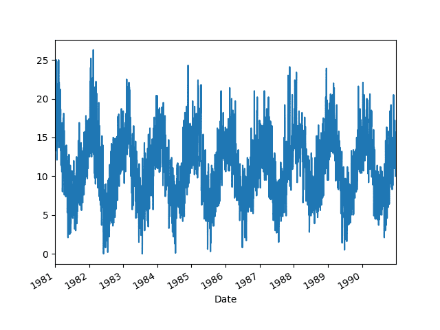
Then the data is graphed as a line plot showing the seasonal pattern.

Minimum Daily Temperatures Dataset Line Plot

ARIMA Forecast Model

In this section, we will fit an ARIMA forecast model to the data.

The parameters of the model will not be tuned, but will be skillful.

The data contains a one-year seasonal component that must be removed to make the data stationary and suitable for use with an ARIMA model.

We can take the seasonal difference by subtracting the observation from one year ago (365 days). This is rough in that it does not account for leap years. It also means that the first year of data will be unavailable for modeling as there is no data one year before to difference the data.

# seasonal difference
differenced = series.diff(365)
# trim off the first year of empty data
differenced = differenced[365:]

# seasonal difference

differenced = series.diff(365)

# trim off the first year of empty data

differenced = differenced[365:]

We will fit an ARIMA(7,0,0) model to the data and print the summary information. This demonstrates that the model is stable.

# fit model
model = ARIMA(differenced, order=(7,0,0))
model_fit = model.fit()
print(model_fit.summary())

# fit model

model = ARIMA(differenced, order=(7,0,0))

model_fit = model.fit()

print(model_fit.summary())

Putting this all together, the complete example is listed below.

# fit an ARIMA model
from pandas import read_csv
from matplotlib import pyplot
from statsmodels.tsa.arima.model import ARIMA
# load dataset
series = read_csv('daily-minimum-temperatures.csv', header=0, index_col=0)
# seasonal difference
differenced = series.diff(365)
# trim off the first year of empty data
differenced = series[365:]
# fit model
model = ARIMA(differenced, order=(7,0,0))
model_fit = model.fit()
print(model_fit.summary())

# fit an ARIMA model

from pandas import read_csv

from matplotlib import pyplot

from statsmodels.tsa.arima.model import ARIMA

# load dataset

series = read_csv('daily-minimum-temperatures.csv', header=0, index_col=0)

# seasonal difference

differenced = series.diff(365)

# trim off the first year of empty data

differenced = series[365:]

# fit model

model = ARIMA(differenced, order=(7,0,0))

model_fit = model.fit()

print(model_fit.summary())

Running the example provides a summary of the fit ARIMA model.

                              ARMA Model Results                              
==============================================================================
Dep. Variable:                   Temp   No. Observations:                 3285
Model:                     ARMA(7, 0)   Log Likelihood               -8690.089
Method:                       css-mle   S.D. of innovations              3.409
Date:                Fri, 25 Aug 2017   AIC                          17396.178
Time:                        15:02:59   BIC                          17444.955
Sample:                    01-01-1982   HQIC                         17413.643
                         - 12-31-1990                                         
==============================================================================
                 coef    std err          z      P>|z|      [0.025      0.975]
------------------------------------------------------------------------------
ar.L1.Temp     0.5278      0.017     30.264      0.000       0.494       0.562
ar.L2.Temp    -0.1099      0.020     -5.576      0.000      -0.149      -0.071
ar.L3.Temp     0.0286      0.020      1.441      0.150      -0.010       0.067
ar.L4.Temp     0.0307      0.020      1.549      0.122      -0.008       0.070
ar.L5.Temp     0.0090      0.020      0.456      0.648      -0.030       0.048
ar.L6.Temp     0.0164      0.020      0.830      0.407      -0.022       0.055
ar.L7.Temp     0.0272      0.017      1.557      0.120      -0.007       0.061
                                    Roots                                    
=============================================================================
                 Real           Imaginary           Modulus         Frequency
-----------------------------------------------------------------------------
AR.1            1.3305           -0.0000j            1.3305           -0.0000
AR.2            0.9936           -1.1966j            1.5553           -0.1397
AR.3            0.9936           +1.1966j            1.5553            0.1397
AR.4           -0.2067           -1.7061j            1.7186           -0.2692
AR.5           -0.2067           +1.7061j            1.7186            0.2692
AR.6           -1.7536           -0.8938j            1.9683           -0.4250
AR.7           -1.7536           +0.8938j            1.9683            0.4250
-----------------------------------------------------------------------------

ARMA Model Results

==============================================================================

Dep. Variable: Temp No. Observations: 3285

Model: ARMA(7, 0) Log Likelihood -8690.089

Method: css-mle S.D. of innovations 3.409

Date: Fri, 25 Aug 2017 AIC 17396.178

Time: 15:02:59 BIC 17444.955

Sample: 01-01-1982 HQIC 17413.643

- 12-31-1990

==============================================================================

coef std err z P>|z| [0.025 0.975]

------------------------------------------------------------------------------

ar.L1.Temp 0.5278 0.017 30.264 0.000 0.494 0.562

ar.L2.Temp -0.1099 0.020 -5.576 0.000 -0.149 -0.071

ar.L3.Temp 0.0286 0.020 1.441 0.150 -0.010 0.067

ar.L4.Temp 0.0307 0.020 1.549 0.122 -0.008 0.070

ar.L5.Temp 0.0090 0.020 0.456 0.648 -0.030 0.048

ar.L6.Temp 0.0164 0.020 0.830 0.407 -0.022 0.055

ar.L7.Temp 0.0272 0.017 1.557 0.120 -0.007 0.061

Roots

=============================================================================

Real Imaginary Modulus Frequency

-----------------------------------------------------------------------------

AR.1 1.3305 -0.0000j 1.3305 -0.0000

AR.2 0.9936 -1.1966j 1.5553 -0.1397

AR.3 0.9936 +1.1966j 1.5553 0.1397

AR.4 -0.2067 -1.7061j 1.7186 -0.2692

AR.5 -0.2067 +1.7061j 1.7186 0.2692

AR.6 -1.7536 -0.8938j 1.9683 -0.4250

AR.7 -1.7536 +0.8938j 1.9683 0.4250

-----------------------------------------------------------------------------

Model History Sensitivity Analysis

In this section, we will explore the effect that history size has on the skill of the fit model.

The original data has 10 years of data. Seasonal differencing leaves us with 9 years of data. We will hold back the final year of data as test data and perform walk-forward validation across this final year.

The day-by-day forecasts will be collected and a root mean squared error (RMSE) score will be calculated to indicate the skill of the model.

The snippet below separates the seasonally adjusted data into training and test datasets.

train, test = differenced[differenced.index < '1990'], differenced['1990']

1	train, test = differenced[differenced.index < '1990'], differenced['1990']

It is important to choose an interval that makes sense for your own forecast problem.

We will evaluate the skill of the model with the previous 1 year of data, then 2 years, all the way back through the 8 available years of historical data.

A year is a good interval to test for this dataset given the seasonal nature of the data, but other intervals could be tested, such as month-wise or multi-year intervals.

The snippet below shows how we can step backwards by year and cumulatively select all available observations.

For example

Test 1: All data in 1989
Test 2: All data in 1988 to 1989

And so on.

# split
train, test = differenced[differenced.index < '1990'], differenced['1990']
years = ['1989', '1988', '1987', '1986', '1985', '1984', '1983', '1982']
for year in years:
	# select data from 'year' cumulative to 1989
	dataset = train[train.index >= year]

# split

train, test = differenced[differenced.index < '1990'], differenced['1990']

years = ['1989', '1988', '1987', '1986', '1985', '1984', '1983', '1982']

for year in years:

# select data from 'year' cumulative to 1989

dataset = train[train.index >= year]

The next step is to evaluate an ARIMA model.

We will use walk-forward validation. This means that a model will be constructed on the selected historic data and forecast the next time step (Jan 1st 1990). The real observation for that time step will be added to the history, a new model constructed, and the next time step predicted.

The forecasts will be collected together and compared to the final year of observations to give an error score. In this case, RMSE will be used as the scores and will be in the same scale as the observations themselves.

# walk forward over time steps in test
values = dataset.values
history = [values[i] for i in range(len(values))]
predictions = list()
test_values = test.values
for t in range(len(test_values)):
	# fit model
	model = ARIMA(history, order=(7,0,0))
	model_fit = model.fit()
	# make prediction
	yhat = model_fit.forecast()[0]
	predictions.append(yhat)
	history.append(test_values[t])
rmse = sqrt(mean_squared_error(test_values, predictions))
print('%s-%s (%d values) RMSE: %.3f' % (years[0], year, len(values), rmse))

# walk forward over time steps in test

values = dataset.values

history = [values[i] for i in range(len(values))]

predictions = list()

test_values = test.values

for t in range(len(test_values)):

# fit model

model = ARIMA(history, order=(7,0,0))

model_fit = model.fit()

# make prediction

yhat = model_fit.forecast()[0]

predictions.append(yhat)

history.append(test_values[t])

rmse = sqrt(mean_squared_error(test_values, predictions))

print('%s-%s (%d values) RMSE: %.3f' % (years[0], year, len(values), rmse))

Putting this all together, the complete example is listed below.

# fit an ARIMA model
from pandas import read_csv
from matplotlib import pyplot
from statsmodels.tsa.arima.model import ARIMA
from sklearn.metrics import mean_squared_error
from math import sqrt
# load dataset
series = read_csv('daily-minimum-temperatures.csv', header=0, index_col=0)
# seasonal difference
differenced = series.diff(365)
# trim off the first year of empty data
differenced = differenced[365:]
# split
train, test = differenced[differenced.index < '1990'], differenced['1990']
years = ['1989', '1988', '1987', '1986', '1985', '1984', '1983', '1982']
for year in years:
	# select data from 'year' cumulative to 1989
	dataset = train[train.index >= year]
	# walk forward over time steps in test
	values = dataset.values
	history = [values[i] for i in range(len(values))]
	predictions = list()
	test_values = test.values
	for t in range(len(test_values)):
		# fit model
		model = ARIMA(history, order=(7,0,0))
		model_fit = model.fit()
		# make prediction
		yhat = model_fit.forecast()[0]
		predictions.append(yhat)
		history.append(test_values[t])
	rmse = sqrt(mean_squared_error(test_values, predictions))
	print('%s-%s (%d values) RMSE: %.3f' % (years[0], year, len(values), rmse))

# fit an ARIMA model

from pandas import read_csv

from matplotlib import pyplot

from statsmodels.tsa.arima.model import ARIMA

from sklearn.metrics import mean_squared_error

from math import sqrt

# load dataset

series = read_csv('daily-minimum-temperatures.csv', header=0, index_col=0)

# seasonal difference

differenced = series.diff(365)

# trim off the first year of empty data

differenced = differenced[365:]

# split

train, test = differenced[differenced.index < '1990'], differenced['1990']

years = ['1989', '1988', '1987', '1986', '1985', '1984', '1983', '1982']

for year in years:

# select data from 'year' cumulative to 1989

dataset = train[train.index >= year]

# walk forward over time steps in test

values = dataset.values

history = [values[i] for i in range(len(values))]

predictions = list()

test_values = test.values

for t in range(len(test_values)):

# fit model

model = ARIMA(history, order=(7,0,0))

model_fit = model.fit()

# make prediction

yhat = model_fit.forecast()[0]

predictions.append(yhat)

history.append(test_values[t])

rmse = sqrt(mean_squared_error(test_values, predictions))

print('%s-%s (%d values) RMSE: %.3f' % (years[0], year, len(values), rmse))

Running the example prints the interval of history, number of observations in the history, and the RMSE skill of the model trained with that history.

The example does take awhile to run as 365 ARIMA models are created for each cumulative interval of historic training data.

1989-1989 (365 values) RMSE: 3.120
1989-1988 (730 values) RMSE: 3.109
1989-1987 (1095 values) RMSE: 3.104
1989-1986 (1460 values) RMSE: 3.108
1989-1985 (1825 values) RMSE: 3.107
1989-1984 (2190 values) RMSE: 3.103
1989-1983 (2555 values) RMSE: 3.099
1989-1982 (2920 values) RMSE: 3.096

1989-1989 (365 values) RMSE: 3.120

1989-1988 (730 values) RMSE: 3.109

1989-1987 (1095 values) RMSE: 3.104

1989-1986 (1460 values) RMSE: 3.108

1989-1985 (1825 values) RMSE: 3.107

1989-1984 (2190 values) RMSE: 3.103

1989-1983 (2555 values) RMSE: 3.099

1989-1982 (2920 values) RMSE: 3.096

The results show that as the size of the available history is increased, there is a decrease in model error, but the trend is not purely linear.

We do see that there may be a point of diminishing returns at 2-3 years. Knowing that you can use fewer years of data is useful in domains where data availability or long model training time is an issue.

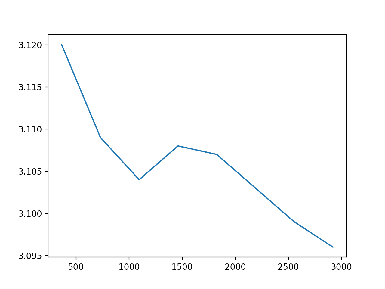
We can plot the relationship between ARIMA model error and the number of training observations.

from matplotlib import pyplot
x = [365, 730, 1095, 1460, 1825, 2190, 2555, 2920]
y = [3.120, 3.109, 3.104, 3.108, 3.107, 3.103, 3.099, 3.096]
pyplot.plot(x, y)
pyplot.show()

from matplotlib import pyplot

x = [365, 730, 1095, 1460, 1825, 2190, 2555, 2920]

y = [3.120, 3.109, 3.104, 3.108, 3.107, 3.103, 3.099, 3.096]

pyplot.plot(x, y)

pyplot.show()

Running the example creates a plot that almost shows a linear trend down in error as training samples increases.

History Size vs ARIMA Model Error

This is generally expected, as more historical data means that the coefficients may be better optimized to describe what happens with the variability from more years of data, for the most part.

There is also a counter-intuition. One may expect the performance of the model to increase with more history, as the data from the most recent years may be more like the data next year. This intuition is perhaps more valid in domains subjected to greater concept drift.

Extensions

This section discusses limitations and extensions to the sensitivity analysis.

Untuned Model. The ARIMA model used in the example is by no means tuned to the problem. Ideally, a sensitivity analysis of the size of training history would be performed with an already tuned ARIMA model or a model tuned to each case.
Statistical Significance. It is not clear whether the difference in model skill is statistically significant. Pairwise statistical significance tests can be used to tease out whether differences in RMSE are meaningful.
Alternate Models. The ARIMA uses historical data to fit coefficients. Other models may use the increasing historical data in other ways. Alternate nonlinear machine learning models may be investigated.
Alternate Intervals. A year was chosen to joint the historical data, but other intervals may be used. A good interval might be weeks or months within one or two years of historical data for this dataset, as the extreme recency may bias the coefficients in useful ways.

Summary

In this tutorial, you discovered how you can design, execute, and analyze a sensitivity analysis of the amount of history used to fit a time series forecast model.

Do you have any questions?
Ask your questions in the comments and I’ll do my best to answer.

21 Responses to Sensitivity Analysis of History Size to Forecast Skill with ARIMA in Python

sura April 7, 2017 at 3:39 am #

thank you ! but, can you give me a download address of dataset? i want to try again!
thank!

Reply
- Jason Brownlee April 9, 2017 at 2:46 pm #
  
  Sorry, here it is:
  https://datamarket.com/data/set/2324/daily-minimum-temperatures-in-melbourne-australia-1981-1990
  
  Reply
Eugeniy May 5, 2017 at 6:44 pm #

Good afternoon!
Thank you for your article.
Tell me please, if there are more formal and mathematical definitions of sensitivity analysis of history size to forecast?
Or is this usually only an experimental way of determining?
Thank you!

Reply
- Jason Brownlee May 6, 2017 at 7:40 am #
  
  I’m sure you can analyze the effect of history size on the model analytically.
  
  A sensitivity analysis seeks to answer the question empirically.
  
  Reply
David Ravnsborg August 18, 2017 at 9:36 am #

Why do you declare “differenced” and then immediately write over it without using it?

Reply
- Jason Brownlee August 18, 2017 at 4:37 pm #
  
  Good question, that looks like a bug to me. I’ll add a note to trello to fix it up.
  
  Reply
  - David Ravnsborg August 18, 2017 at 5:48 pm #
    
    I looked into it a little further on my end. I think it was just a typo where:
    # seasonal difference
    differenced = series.diff(365)
    # trim off the first year of empty data
    differenced = series[365:]
    
    should have been…
    
    # seasonal difference
    differenced = series.diff(365)
    # trim off the first year of empty data
    differenced = differenced[365:]
    
    But it completely changes the results for the worse 🙁 Any chance you could cover this? It would make a great follow-up. Here are the results I get:
    model.py:496: ConvergenceWarning: Maximum Likelihood optimization failed to converge. Check mle_retvals
    “Check mle_retvals”, ConvergenceWarning)
    1989-1989 (365 values) RMSE: 3.120
    1989-1988 (730 values) RMSE: 3.109
    model.py:496: ConvergenceWarning: Maximum Likelihood optimization failed to converge. Check mle_retvals
    “Check mle_retvals”, ConvergenceWarning)
    1989-1987 (1095 values) RMSE: 3.104
    1989-1986 (1460 values) RMSE: 3.108
    1989-1985 (1825 values) RMSE: 3.107
    model.py:496: ConvergenceWarning: Maximum Likelihood optimization failed to converge. Check mle_retvals
    “Check mle_retvals”, ConvergenceWarning)
    1989-1984 (2190 values) RMSE: 3.103
    1989-1983 (2555 values) RMSE: 3.099
    1989-1982 (2920 values) RMSE: 3.096
    
    Reply
    - Jason Brownlee August 25, 2017 at 3:15 pm #
      
      I have updated the post, thanks again David.
      
      We still see the same linearly downward trend in error.
      
      Remember that the RMSE scores are in fact in the units of seasonally differenced temperatures. This may make a difference.
      
      If you’re interested in better results, you can try using a grid search on the ARIMA parameters to see if we can do better than ARIMA(7,0,0) or whether performing a seasonal difference results in better final RMSE on this problem.
      
      Reply
Rahul June 11, 2018 at 7:04 pm #

Hey Jason,

Just a minor edit.

Ctrl+F “The day-by-day forecasts will be collected and a root” and the sentence has been repeated twice. Not an issue but thought you’d like to know.

Awesome posts, I really enjoy reading your work 🙂

Reply
- Jason Brownlee June 12, 2018 at 6:38 am #
  
  Thanks, fixed.
  
  Reply
Raghu October 13, 2018 at 1:16 am #

I checked Stationarity test for the provided dataset using Augmented Dickey-Fuller method and below is the result
Test Statistic -4.445747
p-value 0.000246
#Lags Used 20.000000
Number of Observations Used 3629.000000
Critical Value (1%) -3.432153
Critical Value (5%) -2.862337
Critical Value (10%) -2.567194

based on the result i conclude that data looks very much stationary and
I have a question that even though data is stationary Why did you apply Seasonality dereference ?

Reply
- Jason Brownlee October 13, 2018 at 6:15 am #
  
  What dataset did you evaluate exactly?
  
  The temperature dataset clearly has a time dependent structure.
  
  Reply
  - Raghu October 15, 2018 at 7:24 pm #
    
    I evaluated “daily-minimum-temperatures.csv” dataset (same dataset used in this article).
    but ADF result (copied in last comment) shows data looks stationary.
    
    Reply
lalitha bharathula December 27, 2018 at 10:24 pm #

suppose i want to predict sales in a region based on date and that day temperature( based on temperature like too cold my sales will impact). Please let me know if arima can be used here

Reply
- Jason Brownlee December 28, 2018 at 5:57 am #
  
  Perhaps try it and discover how well it works.
  
  Reply
Btran May 27, 2019 at 7:38 pm #

hi,tks for your blog. i’m newbie, sorry for not good english, can you explain the value in ARIMA model results, i don’t know what the value of AIC, BIC,HQIC and coef,std err,z,P>|z|,…means? And how do know it is a good results?

Reply
- Jason Brownlee May 28, 2019 at 8:12 am #
  
  Good question, perhaps this will help:
  https://machinelearningmastery.com/faq/single-faq/how-to-know-if-a-model-has-good-performance
  
  Reply
Ed November 30, 2019 at 3:38 am #

Great tutorial!. One question about the methodology – you indicated “we can step backwards by year and cumulatively select all available observations”. Is there a reason to step backwards (from 1989 to 1982) instead of stepping forward [from 1982 to 1989, eg. (Test 1) All data in 1982, (Test 2) Test 2: All data in 1982 to 1983, etc.]?

Reply
- Jason Brownlee November 30, 2019 at 6:31 am #
  
  Thanks.
  
  We step forward when evaluating, I was explaining how we expand the window. Sorry for the confusion.
  
  Reply
Diego February 25, 2021 at 9:39 pm #

Hello Jason.

Do you have, any example using logarithm on the time series?

Reply
- Jason Brownlee February 26, 2021 at 4:58 am #
  
  Yes, right here:
  https://machinelearningmastery.com/power-transform-time-series-forecast-data-python/
  
  Reply

Navigation

Sensitivity Analysis of History Size to Forecast Skill with ARIMA in Python

Minimum Daily Temperatures Dataset

ARIMA Forecast Model

Model History Sensitivity Analysis

Extensions

Summary

Want to Develop Time Series Forecasts with Python?

Develop Your Own Forecasts in Minutes

Finally Bring Time Series Forecasting to
Your Own Projects

More On This Topic

21 Responses to Sensitivity Analysis of History Size to Forecast Skill with ARIMA in Python

Leave a Reply Click here to cancel reply.

Navigation

Minimum Daily Temperatures Dataset

ARIMA Forecast Model

Model History Sensitivity Analysis

Extensions

Summary

Want to Develop Time Series Forecasts with Python?

Develop Your Own Forecasts in Minutes

Finally Bring Time Series Forecasting to Your Own Projects

More On This Topic

21 Responses to Sensitivity Analysis of History Size to Forecast Skill with ARIMA in Python

Leave a Reply Click here to cancel reply.

Finally Bring Time Series Forecasting to
Your Own Projects