A better first-cut forecast on time series data with a seasonal component is to persist the observation for the same time in the previous season. This is called seasonal persistence.
In this tutorial, you will discover how to implement seasonal persistence for time series forecasting in Python.
After completing this tutorial, you will know:
How to use point observations from prior seasons for a persistence forecast.
How to use mean observations across a sliding window of prior seasons for a persistence forecast.
How to apply and evaluate seasonal persistence on monthly and daily time series data.
Kick-start your project with my new book Time Series Forecasting With Python, including step-by-step tutorials and the Python source code files for all examples.
Let’s get started.
Updated Apr/2019: Updated the links to datasets.
Updated Aug/2019: Updated data loading to use new API.
Seasonal Persistence
It is critical to have a useful first-cut forecast on time series problems to provide a lower-bound on skill before moving on to more sophisticated methods.
This is to ensure we are not wasting time on models or datasets that are not predictive.
It is common to use a persistence or a naive forecast as a first-cut forecast model when time series forecasting.
This does not make sense with time series data that has an obvious seasonal component. A better first cut model for seasonal data is to use the observation at the same time in the previous seasonal cycle as the prediction.
We can call this “seasonal persistence” and it is a simple model that can result in an effective first cut model.
One step better is to use a simple function of the last few observations at the same time in previous seasonal cycles. For example, the mean of the observations. This can often provide a small additional benefit.
In this tutorial, we will demonstrate this simple seasonal persistence forecasting method for providing a lower bound on forecast skill on three different real-world time series datasets.
Seasonal Persistence with Sliding Window
In this tutorial, we will use a sliding window seasonal persistence model to make forecasts.
Within a sliding window, observations at the same time in previous one-year seasons will be collected and the mean of those observations can be used as the persisted forecast.
Different window sizes can be evaluated to find a combination that minimizes error.
As an example, if the data is monthly and the month to be predicted is February, then with a window of size 1 (w=1) the observation last February will be used to make the forecast.
A window of size 2 (w=2) would involve taking observations for the last two Februaries to be averaged and used as a forecast.
An alternate interpretation might seek to use point observations from prior years (e.g. t-12, t-24, etc. for monthly data) rather than taking the mean of the cumulative point observations. Perhaps try both methods on your dataset and see what works best as a good starting point model.
Stop learning Time Series Forecasting the slow way!
Take my free 7-day email course and discover how to get started (with sample code).
Click to sign-up and also get a free PDF Ebook version of the course.
Experimental Test Harness
It is important to evaluate time series forecasting models consistently.
In this section, we will define how we will evaluate forecast models in this tutorial.
First, we will hold the last two years of data back and evaluate forecasts on this data. This works for both monthly and daily data we will look at.
We will use a walk-forward validation to evaluate model performance. This means that each time step in the test dataset will be enumerated, a model constructed on historical data, and the forecast compared to the expected value. The observation will then be added to the training dataset and the process repeated.
Walk-forward validation is a realistic way to evaluate time series forecast models as one would expect models to be updated as new observations are made available.
Finally, forecasts will be evaluated using root mean squared error, or RMSE. The benefit of RMSE is that it penalizes large errors and the scores are in the same units as the forecast values (car sales per month).
In summary, the test harness involves:
The last 2 years of data used as a test set.
Walk-forward validation for model evaluation.
Root mean squared error used to report model skill.
Case Study 1: Monthly Car Sales Dataset
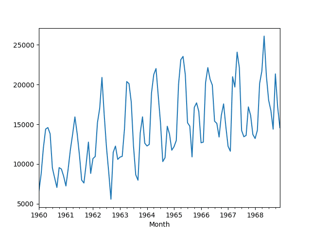
The Monthly Car Sales dataset describes the number of car sales in Quebec, Canada between 1960 and 1968.
The units are a count of the number of sales and there are 108 observations. The source of the data is credited to Abraham and Ledolter (1983).
Download the dataset and save it into your current working directory with the filename “car-sales.csv“. Note, you may need to delete the footer information from the file.
The code below loads the dataset as a Pandas Series object.
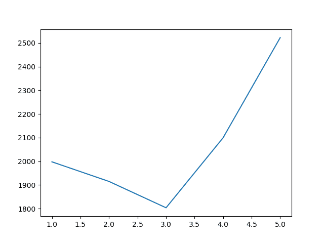
Running the example prints the year number and the RMSE for the mean observation from the sliding window of observations at the same month in prior years.
The results suggest that taking the average from the last three years is a good starting model with an RMSE of 1803.630 car sales.
1
2
3
4
5
Years=1, RMSE: 1997.732
Years=2, RMSE: 1914.911
Years=3, RMSE: 1803.630
Years=4, RMSE: 2099.481
Years=5, RMSE: 2522.235
A plot of the relationship of sliding window size to model error is created.
The plot nicely shows the improvement with the sliding window size to 3 years, then the rapid increase in error from that point.
Sliding Window Size to RMSE for Monthly Car Sales
Case Study 2: Monthly Writing Paper Sales Dataset
The Monthly Writing Paper Sales dataset describes the number of specialty writing paper sales.
The units are a type of count of the number of sales and there are 147 months of observations (just over 12 years). The counts are fractional, suggesting the data may in fact be in the units of hundreds of thousands of sales. The source of the data is credited to Makridakis and Wheelwright (1989).
Download the dataset and save it into your current working directory with the filename “writing-paper-sales.csv“. Note, you may need to delete the footer information from the file.
The date-time stamps only contain the year number and month. Therefore, a custom date-time parsing function is required to load the data and base the data in an arbitrary year. The year 1900 was chosen as the starting point, which should not affect this case study.
The example below loads the Monthly Writing Paper Sales dataset as a Pandas Series.
Running the example prints the first 5 rows of the loaded dataset.
1
2
3
4
5
6
Month
1901-01-01 1359.795
1901-02-01 1278.564
1901-03-01 1508.327
1901-04-01 1419.710
1901-05-01 1440.510
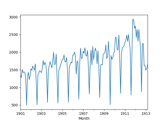
A line plot of the loaded dataset is then created. We can see the yearly seasonal component and an increasing trend.
Line Plot of Monthly Writing Paper Sales Dataset
As in the previous example, we can hold back the last 24 months of observations as a test dataset. Because we have much more data, we will try sliding window sizes from 1 year to 10 years.
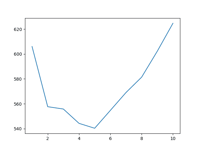
Running the example prints the size of the sliding window and the resulting seasonal persistence model error.
The results suggest that a window size of 5 years is optimal, with an RMSE of 554.660 monthly writing paper sales.
1
2
3
4
5
6
7
8
9
10
Years=1, RMSE: 606.089
Years=2, RMSE: 557.653
Years=3, RMSE: 555.777
Years=4, RMSE: 544.251
Years=5, RMSE: 540.317
Years=6, RMSE: 554.660
Years=7, RMSE: 569.032
Years=8, RMSE: 581.405
Years=9, RMSE: 602.279
Years=10, RMSE: 624.756
The relationship between window size and error is graphed on a line plot showing a similar trend in error to the previous scenario. Error drops to an inflection point (in this case 5 years) before increasing again.
Sliding Window Size to RMSE for Monthly Writing Paper Sales
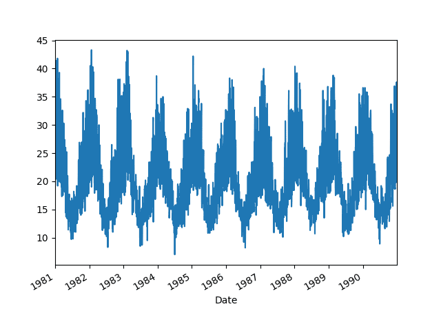
Case Study 3: Daily Maximum Melbourne Temperatures Dataset
The Daily Maximum Melbourne Temperatures dataset describes the daily temperatures in the city Melbourne, Australia from 1981 to 1990.
The units are in degrees Celsius and there 3,650 observations, or 10 years of data. The source of the data is credited to the Australian Bureau of Meteorology.
Download the dataset and save it into your current working directory with the filename “max-daily-temps.csv“. Note, you may need to delete the footer information from the file.
The example below demonstrates loading the dataset as a Pandas Series.
Running the example prints the first 5 rows of data.
1
2
3
4
5
6
Date
1981-01-01 38.1
1981-01-02 32.4
1981-01-03 34.5
1981-01-04 20.7
1981-01-05 21.5
A line plot is also created. We can see we have a lot more observations than the previous two scenarios and that there is a clear seasonal trend in the data.
Line Plot of Daily Melbourne Maximum Temperatures Dataset
Because the data is daily, we need to specify the years in the test data as a function of 365 days rather than 12 months.
This ignores leap years, which is a complication that could, or even should, be addressed in your own project.
The complete example of seasonal persistence is listed below.
Running the example prints the size of the sliding window and the corresponding model error.
Unlike the previous two cases, we can see a trend where the skill continues to improve as the window size is increased.
The best result is a sliding window of all 8 years of historical data with an RMSE of 4.271.
1
2
3
4
5
6
7
8
Years=1, RMSE: 5.950
Years=2, RMSE: 5.083
Years=3, RMSE: 4.664
Years=4, RMSE: 4.539
Years=5, RMSE: 4.448
Years=6, RMSE: 4.358
Years=7, RMSE: 4.371
Years=8, RMSE: 4.271
The plot of sliding window size to model error makes this trend apparent.
It suggests that getting more historical data for this problem might be useful if an optimal model turns out to be a function of the observations on the same day in prior years.
Sliding Window Size to RMSE for Daily Melbourne Maximum Temperature
We might do just as well if the observations were averaged from the same week or month in previous seasons, and this might prove a fruitful experiment.
Summary
In this tutorial, you discovered seasonal persistence for time series forecasting.
You learned:
How to use point observations from prior seasons for a persistence forecast.
How to use a mean of a sliding window across multiple prior seasons for a persistence forecast.
How to apply seasonal persistence to daily and monthly time series data.
Do you have any questions about persistence with seasonal data?
Ask your questions in the comments and I will do my best to answer.
Want to Develop Time Series Forecasts with Python?
The first example – history.append(test[i]), you are mutating the history list in a loop. This is a horrible way of coding. Instead, you should manipulate the index.
And your program is not correct. This is the correct versoin
from pandas import Series
from sklearn.metrics import mean_squared_error
from math import sqrt
from numpy import mean
from matplotlib import pyplot
# load data
series = Series.from_csv(‘car-sales.csv’, header=0)
# prepare data
X = series.values
train, test = X[0:-24], X[-24:]
# evaluate mean of different number of years
years = [1, 2, 3, 4, 5]
scores = list()
for year in years:
# walk-forward validation
predictions = list()
for i in range(len(test)):
# collect obs
obs = list()
for y in range(1, year+1):
obs.append(train[-y*12 + i])
# make prediction
yhat = mean(obs)
predictions.append(yhat)
Thank you for this tutorial, and tying together data models from previous posts. Providing a means to evaluate seasonal persistence with a sliding windows, and then graphing the results is dynamite mate.
I really like the format of Introduction, Test Harness, Case Studies, and Summary. It helps me draw a real world connection with the data set.
First of all, I’ve learned a lot from your tutorials. I’d like to say “thank you”.
As to the examples in this tutorial, there was a comment made back in April by “x” who didn’t elaborate where he thought the programs had mistakes as requested. I think the mistake is in line 22 of the complete code of the 1st example:
obs.append(history[-(y*12)])
I think this line should be:
obs.append(history[-(y*12 + i)])
because we want to collect the figures of the ith month over the last few years represented by y.
All the other examples seem to have the same problem.
I was stuck on this too. Jason’s code is correct. The reason you don’t need obs.append(history[-(y*12 + i)]) is because he is appending history with the test[i].
@ Jason Thanks for such a detailed walk through the model. Really helpful and easy to understand.
One question – how can I use this seasonal method to produce forecasts for multistep out-of-time future data (that is not part of the input data). …Lets say I am looking to use this to produce 12 immediate next data points….
My future work is to forecast weather for the future year(s). For Now I have read about some time series models like ARIMA, MA aswell as AR models and there are also other weather forecasting models like ETS that can be used in this domain.
My first question is, I wish to know if you have any idea regarding the “classic” models which have been used in the past and today for weather forecasting. Thank you in advance for ur time and response.
I also wish to find out if your Ebook on time series is also available in hard copy. By the way is the EBook free? I saw something like $37 online. Could it be for the Ebook or the hard copy(if available).
Thanks alot for you quick reply. Also as I said previosly, I recently read ARIMA models can be used for forecasting.
I wish to ask if you know any of the “classic” (Standard models generally used in different countries to predict weather ) which have been used in the past and today for weather forecasting.
Very useful post! I just have one follow up question – how would you compute a 95% confidence interval for the forecasted values if the forecasts are equal to the mean of a sliding window across multiple prior seasons? Note that I am working with monthly data. Thanks in advance for your help.


The first example – history.append(test[i]), you are mutating the history list in a loop. This is a horrible way of coding. Instead, you should manipulate the index.
And your program is not correct. This is the correct versoin
from pandas import Series
from sklearn.metrics import mean_squared_error
from math import sqrt
from numpy import mean
from matplotlib import pyplot
# load data
series = Series.from_csv(‘car-sales.csv’, header=0)
# prepare data
X = series.values
train, test = X[0:-24], X[-24:]
# evaluate mean of different number of years
years = [1, 2, 3, 4, 5]
scores = list()
for year in years:
# walk-forward validation
predictions = list()
for i in range(len(test)):
# collect obs
obs = list()
for y in range(1, year+1):
obs.append(train[-y*12 + i])
# make prediction
yhat = mean(obs)
predictions.append(yhat)
# report performance
rmse = sqrt(mean_squared_error(test, predictions))
scores.append(rmse)
print(‘Years=%d, RMSE: %.3f’ % (year, rmse))
pyplot.plot(years, scores)
pyplot.show()
Can you elaborate on the fault you believe you have discovered and fixed?
I do not agree. This is a fine way of demonstrating walk forward validation.
It makes no sense the accuracy of using 5 years data is the worst as the chart you printed out for the first example.
I believe you have misread the example.
We use RMSE not accuracy and RMSE was best (lowest) with the maximum amount of history.
Thank you for this tutorial, and tying together data models from previous posts. Providing a means to evaluate seasonal persistence with a sliding windows, and then graphing the results is dynamite mate.
I really like the format of Introduction, Test Harness, Case Studies, and Summary. It helps me draw a real world connection with the data set.
I’m very grateful for your site.
Thanks Jordan, I’m really glad to hear that.
First of all, I’ve learned a lot from your tutorials. I’d like to say “thank you”.
As to the examples in this tutorial, there was a comment made back in April by “x” who didn’t elaborate where he thought the programs had mistakes as requested. I think the mistake is in line 22 of the complete code of the 1st example:
obs.append(history[-(y*12)])
I think this line should be:
obs.append(history[-(y*12 + i)])
because we want to collect the figures of the ith month over the last few years represented by y.
All the other examples seem to have the same problem.
Thanks for the note.
I was stuck on this too. Jason’s code is correct. The reason you don’t need obs.append(history[-(y*12 + i)]) is because he is appending history with the test[i].
Thanks Scott.
@ Jason Thanks for such a detailed walk through the model. Really helpful and easy to understand.
One question – how can I use this seasonal method to produce forecasts for multistep out-of-time future data (that is not part of the input data). …Lets say I am looking to use this to produce 12 immediate next data points….
Thanks so much
You can walk the method forward, even use predictions as observations as required.
@ Jason, wrt my previous note, never mind..that was a silly question..i could do it myself 🙂
No problem.
Hello Jason,
My future work is to forecast weather for the future year(s). For Now I have read about some time series models like ARIMA, MA aswell as AR models and there are also other weather forecasting models like ETS that can be used in this domain.
My first question is, I wish to know if you have any idea regarding the “classic” models which have been used in the past and today for weather forecasting. Thank you in advance for ur time and response.
I also wish to find out if your Ebook on time series is also available in hard copy. By the way is the EBook free? I saw something like $37 online. Could it be for the Ebook or the hard copy(if available).
Best regards
Goddy
I recommend testing a range of different models on your dataset and see what works best for your specific dataset.
Sorry, I only sell ebooks, I don’t have hard copies.
You can access my best free tutorials on time series here:
https://machinelearningmastery.com/start-here/#timeseries
Thanks alot for you quick reply. Also as I said previosly, I recently read ARIMA models can be used for forecasting.
I wish to ask if you know any of the “classic” (Standard models generally used in different countries to predict weather ) which have been used in the past and today for weather forecasting.
Thanks in advance for your reply
I believe they run simulations of physical processes instead of linear forecasting models.
Very useful post! I just have one follow up question – how would you compute a 95% confidence interval for the forecasted values if the forecasts are equal to the mean of a sliding window across multiple prior seasons? Note that I am working with monthly data. Thanks in advance for your help.
Perhaps the 2x the standard deviation of the sliding window?
https://en.wikipedia.org/wiki/68%E2%80%9395%E2%80%9399.7_rule