
Moving average smoothing is a naive and effective technique in time series forecasting.
It can be used for data preparation, feature engineering, and even directly for making predictions.
In this tutorial, you will discover how to use moving average smoothing for time series forecasting with Python.
After completing this tutorial, you will know:
- How moving average smoothing works and some expectations of your data before you can use it.
- How to use moving average smoothing for data preparation and feature engineering.
- How to use moving average smoothing to make predictions.
Kick-start your project with my new book Time Series Forecasting With Python, including step-by-step tutorials and the Python source code files for all examples.
Let’s get started.
- Updated Apr/2019: Updated the link to dataset.
- Updated Aug/2019: Updated data loading to use new API.

Moving Average Smoothing for Data Preparation, Feature Engineering, and Time Series Forecasting with Python
Photo by Bureau of Land Management, some rights reserved.
Moving Average Smoothing
Smoothing is a technique applied to time series to remove the fine-grained variation between time steps.
The hope of smoothing is to remove noise and better expose the signal of the underlying causal processes. Moving averages are a simple and common type of smoothing used in time series analysis and time series forecasting.
Calculating a moving average involves creating a new series where the values are comprised of the average of raw observations in the original time series.
A moving average requires that you specify a window size called the window width. This defines the number of raw observations used to calculate the moving average value.
The “moving” part in the moving average refers to the fact that the window defined by the window width is slid along the time series to calculate the average values in the new series.
There are two main types of moving average that are used: Centered and Trailing Moving Average.
Centered Moving Average
The value at time (t) is calculated as the average of raw observations at, before, and after time (t).
For example, a center moving average with a window of 3 would be calculated as:
|
1 |
center_ma(t) = mean(obs(t-1), obs(t), obs(t+1)) |
This method requires knowledge of future values, and as such is used on time series analysis to better understand the dataset.
A center moving average can be used as a general method to remove trend and seasonal components from a time series, a method that we often cannot use when forecasting.
Trailing Moving Average
The value at time (t) is calculated as the average of the raw observations at and before the time (t).
For example, a trailing moving average with a window of 3 would be calculated as:
|
1 |
trail_ma(t) = mean(obs(t-2), obs(t-1), obs(t)) |
Trailing moving average only uses historical observations and is used on time series forecasting.
It is the type of moving average that we will focus on in this tutorial.
Data Expectations
Calculating a moving average of a time series makes some assumptions about your data.
It is assumed that both trend and seasonal components have been removed from your time series.
This means that your time series is stationary, or does not show obvious trends (long-term increasing or decreasing movement) or seasonality (consistent periodic structure).
There are many methods to remove trends and seasonality from a time series dataset when forecasting. Two good methods for each are to use the differencing method and to model the behavior and explicitly subtract it from the series.
Moving average values can be used in a number of ways when using machine learning algorithms on time series problems.
In this tutorial, we will look at how we can calculate trailing moving average values for use as data preparation, feature engineering, and for directly making predictions.
Before we dive into these examples, let’s look at the Daily Female Births dataset that we will use in each example.
Stop learning Time Series Forecasting the slow way!
Take my free 7-day email course and discover how to get started (with sample code).
Click to sign-up and also get a free PDF Ebook version of the course.
Daily Female Births Dataset
This dataset describes the number of daily female births in California in 1959.
The units are a count and there are 365 observations. The source of the dataset is credited to Newton (1988).
Below is a sample of the first 5 rows of data, including the header row.
|
1 2 3 4 5 6 |
"Date","Births" "1959-01-01",35 "1959-01-02",32 "1959-01-03",30 "1959-01-04",31 "1959-01-05",44 |
Below is a plot of the entire dataset.
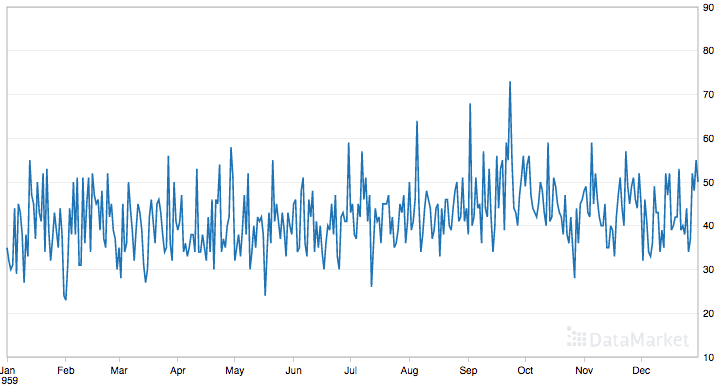
Daily Female Births Dataset
This dataset is a good example for exploring the moving average method as it does not show any clear trend or seasonality.
Load the Daily Female Births Dataset
Download the dataset and place it in the current working directory with the filename “daily-total-female-births.csv“.
The snippet below loads the dataset as a Series, displays the first 5 rows of the dataset, and graphs the whole series as a line plot.
|
1 2 3 4 5 6 |
from pandas import read_csv from matplotlib import pyplot series = read_csv('daily-total-female-births.csv', header=0, index_col=0) print(series.head()) series.plot() pyplot.show() |
Running the example prints the first 5 rows as follows:
|
1 2 3 4 5 6 |
Date 1959-01-01 35 1959-01-02 32 1959-01-03 30 1959-01-04 31 1959-01-05 44 |
Below is the displayed line plot of the loaded data.
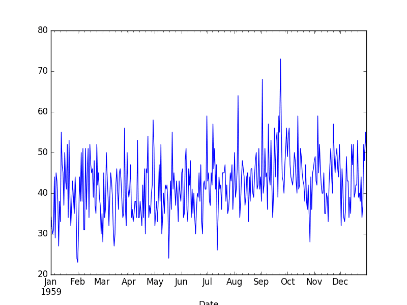
Daily Female Births Dataset Plot
Moving Average as Data Preparation
Moving average can be used as a data preparation technique to create a smoothed version of the original dataset.
Smoothing is useful as a data preparation technique as it can reduce the random variation in the observations and better expose the structure of the underlying causal processes.
The rolling() function on the Series Pandas object will automatically group observations into a window. You can specify the window size, and by default a trailing window is created. Once the window is created, we can take the mean value, and this is our transformed dataset.
New observations in the future can be just as easily transformed by keeping the raw values for the last few observations and updating a new average value.
To make this concrete, with a window size of 3, the transformed value at time (t) is calculated as the mean value for the previous 3 observations (t-2, t-1, t), as follows:
|
1 |
obs(t) = 1/3 * (t-2 + t-1 + t) |
For the Daily Female Births dataset, the first moving average would be on January 3rd, as follows:
|
1 2 3 |
obs(t) = 1/3 * (t-2 + t-1 + t) obs(t) = 1/3 * (35 + 32 + 30) obs(t) = 32.333 |
Below is an example of transforming the Daily Female Births dataset into a moving average with a window size of 3 days, chosen arbitrarily.
|
1 2 3 4 5 6 7 8 9 10 11 |
from pandas import read_csv from matplotlib import pyplot series = read_csv('daily-total-female-births.csv', header=0, index_col=0) # Tail-rolling average transform rolling = series.rolling(window=3) rolling_mean = rolling.mean() print(rolling_mean.head(10)) # plot original and transformed dataset series.plot() rolling_mean.plot(color='red') pyplot.show() |
Running the example prints the first 10 observations from the transformed dataset.
We can see that the first 2 observations will need to be discarded.
|
1 2 3 4 5 6 7 8 9 10 11 |
Date 1959-01-01 NaN 1959-01-02 NaN 1959-01-03 32.333333 1959-01-04 31.000000 1959-01-05 35.000000 1959-01-06 34.666667 1959-01-07 39.333333 1959-01-08 39.000000 1959-01-09 42.000000 1959-01-10 36.000000 |
The raw observations are plotted (blue) with the moving average transform overlaid (red).
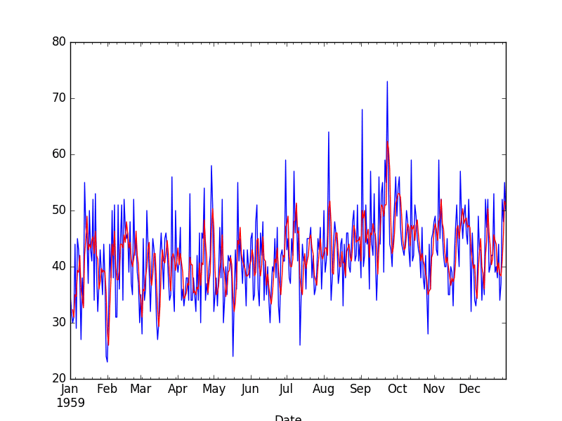
Moving Average Transform
To get a better idea of the effect of the transform, we can zoom in and plot the first 100 observations.
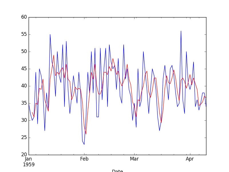
Zoomed Moving Average Transform
Here, you can clearly see the lag in the transformed dataset.
Next, let’s take a look at using the moving average as a feature engineering method.
Moving Average as Feature Engineering
The moving average can be used as a source of new information when modeling a time series forecast as a supervised learning problem.
In this case, the moving average is calculated and added as a new input feature used to predict the next time step.
First, a copy of the series must be shifted forward by one time step. This will represent the input to our prediction problem, or a lag=1 version of the series. This is a standard supervised learning view of the time series problem. For example:
|
1 2 3 4 |
X, y NaN, obs1 obs1, obs2 obs2, obs3 |
Next, a second copy of the series needs to be shifted forward by one, minus the window size. This is to ensure that the moving average summarizes the last few values and does not include the value to be predicted in the average, which would be an invalid framing of the problem as the input would contain knowledge of the future being predicted.
For example, with a window size of 3, we must shift the series forward by 2 time steps. This is because we want to include the previous two observations as well as the current observation in the moving average in order to predict the next value. We can then calculate the moving average from this shifted series.
Below is an example of how the first 5 moving average values are calculated. Remember, the dataset is shifted forward 2 time steps and as we move along the time series, it takes at least 3 time steps before we even have enough data to calculate a window=3 moving average.
|
1 2 3 4 5 6 |
Observations, Mean NaN NaN NaN, NaN NaN NaN, NaN, 35 NaN NaN, 35, 32 NaN 30, 32, 35 32 |
Below is an example of including the moving average of the previous 3 values as a new feature, as wellas a lag-1 input feature for the Daily Female Births dataset.
|
1 2 3 4 5 6 7 8 9 10 11 12 13 |
from pandas import read_csv from pandas import DataFrame from pandas import concat series = read_csv('daily-total-female-births.csv', header=0, index_col=0) df = DataFrame(series.values) width = 3 lag1 = df.shift(1) lag3 = df.shift(width - 1) window = lag3.rolling(window=width) means = window.mean() dataframe = concat([means, lag1, df], axis=1) dataframe.columns = ['mean', 't-1', 't+1'] print(dataframe.head(10)) |
Running the example creates the new dataset and prints the first 10 rows.
We can see that the first 3 rows cannot be used and must be discarded. The first row of the lag1 dataset cannot be used because there are no previous observations to predict the first observation, therefore a NaN value is used.
|
1 2 3 4 5 6 7 8 9 10 11 |
mean t-1 t+1 0 NaN NaN 35 1 NaN 35.0 32 2 NaN 32.0 30 3 NaN 30.0 31 4 32.333333 31.0 44 5 31.000000 44.0 29 6 35.000000 29.0 45 7 34.666667 45.0 43 8 39.333333 43.0 38 9 39.000000 38.0 27 |
The next section will look at how to use the moving average as a naive model to make predictions.
Moving Average as Prediction
The moving average value can also be used directly to make predictions.
It is a naive model and assumes that the trend and seasonality components of the time series have already been removed or adjusted for.
The moving average model for predictions can easily be used in a walk-forward manner. As new observations are made available (e.g. daily), the model can be updated and a prediction made for the next day.
We can implement this manually in Python. Below is an example of the moving average model used in a walk-forward manner.
|
1 2 3 4 5 6 7 8 9 10 11 12 13 14 15 16 17 18 19 20 21 22 23 24 25 26 27 28 29 |
from pandas import read_csv from numpy import mean from sklearn.metrics import mean_squared_error from matplotlib import pyplot series = read_csv('daily-total-female-births.csv', header=0, index_col=0) # prepare situation X = series.values window = 3 history = [X[i] for i in range(window)] test = [X[i] for i in range(window, len(X))] predictions = list() # walk forward over time steps in test for t in range(len(test)): length = len(history) yhat = mean([history[i] for i in range(length-window,length)]) obs = test[t] predictions.append(yhat) history.append(obs) print('predicted=%f, expected=%f' % (yhat, obs)) error = mean_squared_error(test, predictions) print('Test MSE: %.3f' % error) # plot pyplot.plot(test) pyplot.plot(predictions, color='red') pyplot.show() # zoom plot pyplot.plot(test[0:100]) pyplot.plot(predictions[0:100], color='red') pyplot.show() |
Running the example prints the predicted and expected value each time step moving forward, starting from time step 4 (1959-01-04).
Finally, the mean squared error (MSE) is reported for all predictions made.
|
1 2 3 4 5 6 7 8 9 10 11 |
predicted=32.333333, expected=31.000000 predicted=31.000000, expected=44.000000 predicted=35.000000, expected=29.000000 predicted=34.666667, expected=45.000000 predicted=39.333333, expected=43.000000 ... predicted=38.333333, expected=52.000000 predicted=41.000000, expected=48.000000 predicted=45.666667, expected=55.000000 predicted=51.666667, expected=50.000000 Test MSE: 61.379 |
The example ends by plotting the expected test values (blue) compared to the predictions (red).
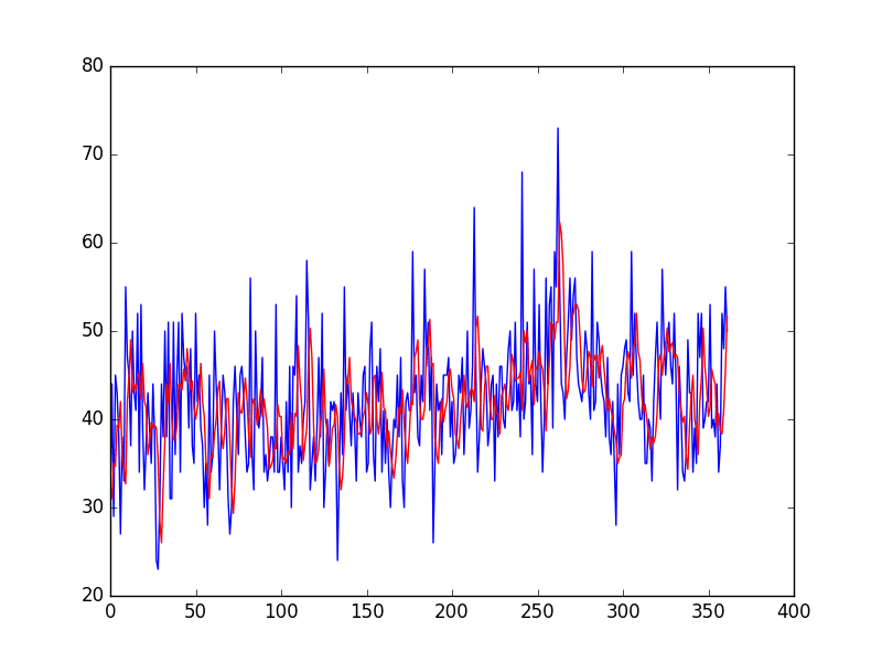
Moving Average Predictions
Again, zooming in on the first 100 predictions gives an idea of the skill of the 3-day moving average predictions.
Note the window width of 3 was chosen arbitrary and was not optimized.
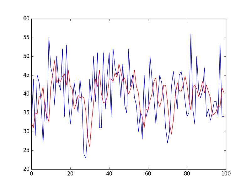
Zoomed Moving Average Predictions
Further Reading
This section lists some resources on smoothing moving averages for time series analysis and time series forecasting that you may find useful.
- Chapter 4, Smoothing Methods, Practical Time Series Forecasting with R: A Hands-On Guide.
- Section 1.5.4 Smoothing, Introductory Time Series with R.
- Section 2.4 Smoothing in the Time Series Context, Time Series Analysis and Its Applications: With R Examples.
Summary
In this tutorial, you discovered how to use moving average smoothing for time series forecasting with Python.
Specifically, you learned:
- How moving average smoothing works and the expectations of time series data before using it.
- How to use moving average smoothing for data preparation in Python.
- How to use moving average smoothing for feature engineering in Python.
- How to use moving average smoothing to make predictions in Python.
Do you have any questions about moving average smoothing, or about this tutorial?
Ask your questions in the comments below and I will do my best to answer.
Want to Develop Time Series Forecasts with Python?

Develop Your Own Forecasts in Minutes
...with just a few lines of python codeDiscover how in my new Ebook:
Introduction to Time Series Forecasting With Python
It covers self-study tutorials and end-to-end projects on topics like: Loading data, visualization, modeling, algorithm tuning, and much more...
Finally Bring Time Series Forecasting to
Your Own Projects
Skip the Academics. Just Results.


Hello,
thank you for all the articles and books, they are great.
Here I am not sure about one thing. Is the
shift(width - 1)correct? In this code:width = 3
lag1 = df.shift(1)
lag3 = df.shift(width – 1)
I think it should be always
shift(2), no matter what is the width, because we do the shift to skip only one single current value (so it is not included in the window later).For example for an input series df=[1,2,3,4,5,6,7] and width=4 there will be
shift(3)that leads to:t t+1 shift(3) mean
– 1 – –
1 2 – –
2 3 – –
3 4 1 –
4 5 2 –
5 6 3 –
6 7 4 2,5
but the mean 2,5 belongs to t=5, not t=6, right?
But of course maybe I just didn’t understand it correctly.
Sounds reasonable Petr.
What if dataset does not continuous sequences, meaning observations for some days are missing. In that case will rolling function be able to identify discontinuous sequences and create mean accordingly?
This post offers some ideas:
https://machinelearningmastery.com/handle-missing-timesteps-sequence-prediction-problems-python/
I am surprised you do not have pd.rolling_apply because some people might want rolling standard deviation or time domain statistics. “A robust, real-time control scheme for multifunction myoelectric control”
Great suggestion, thanks!
I would like to piggyback onto Petr’s comment and say that I believe what is desired is a change from this
lag1 = df.shift(1)
to this
lag1 = df.shift(window – 2)
I also agree with him in that your tutorial’s are great.
Thanks Matt.
Great article. I am trying to use it with a CPU utilization of a node. I am interested in finding out how long usage stayed at 90% or higher. How can I achieve it. Can you please provide some pointer.
No idea, sorry.
Great article….
if ynew == 2:
print (“a movement is Identified”)
else:
print (“Stable Condition”)
time.sleep(0.5)
how can I take moving average on (ynew== 2) in this condition.
I don’t follow sorry, what do you mean exactly?
In the case of trailing moving average calculation, why do we need to shift the data? I mean, the rolling window will always be based on the current and past value, not the future values. So, even without shifting the data, wouldn’t we get valid results? In the case above, we would get valid mean from index 2 (in the feature engineering section).
Am I missing something?
Shifting has to do with transforming a sequence into a supervised learning problem:
https://machinelearningmastery.com/time-series-forecasting-supervised-learning/
Speaking of shifting-time, I think you can help my current work about forecasting time series with Generalized Linear Model. The reason why I use GLM method is I consider temperature (T(t),T(t-1),…), rainfall (R(t),R(t-1),…), humidity (H(t),H(t-1),…), and past event (Y(t-1),…) as the explanatory variables to current event (Y(t)). Let’s say Y(t)~T(t)+R(t)+H(t)+Y(t-1)+T(t-1)+R(t-1)+H(t-1) for lag-1. By comparing plots, I can see that my prediction at time t consistently more looks alike the real obervation at time t-1. I say it’s like shifting (delay) one time-step. I have no idea why this is happening. I think it’s related to “time series” as random walk process. Can you explain me why? Thank you in advance, Jason. I’m a student by the way, so I do really appreciate your help.
It may suggest your model has learned a persistance forecast:
https://machinelearningmastery.com/faq/single-faq/why-is-my-forecasted-time-series-right-behind-the-actual-time-series
Hey, how do you decide on the window size in a time series data? Is there any publication on this front that I can refer to?
Empirical evaluation.
Test a suite of window sizes and see what works well.best on your specific dataset.
Hi professor thanks for this priceless knowledge you impart on here . For a moving average as one of the features to an LSTM model. Do I need to still remove trend or seasonality?
And does this work
MA30 = data[‘close’].rolling(30).mean().
I thought that should work for moving average and also for .var.
Assuming there was already a dataset with close as a column for closing price.
Thank you
Yes, it would be a good idea to make the series stationary first.
1 doubt from the above article. Kindly reply.
> A center moving average can be used as a general method to remove trend and seasonal components from a time series, a method that we often cannot use when forecasting.
> It is a naive model (for prediction) and assumes that the trend and seasonality components of the time series have already been removed or adjusted for.
1) Why to remove trend and seasonality components for prediction?
2) If seasonality has to be removed before forecasting, then why center moving average cannot be used? As per the above article, center moving average would remove seasonality!
Removing the trend and seasonality can make the series stationary and easier to model:
https://machinelearningmastery.com/time-series-data-stationary-python/
Moving average may not remove seasonality.
Thanks for the article, it’s so enlighthening
just interesting the smoothing with moving average for the data preparation.
let say later on, it will use certain algorithm to make prediction.
whether the smoothing applied to the whole raw data or for training dataset only?
All input to the model, training and any new data that is fed in.
When I average the dataset every 60 seconds, it becomes a dataset every minute. When some important information is hidden in seconds, but it disappears after averaging every minute, how can I use the information of seconds to improve the prediction every minute? Thank you
It can smooth out the variance seen at the “seconds” level of detail. It may or may not help – depends on your data and choice of model.
Hi Jason, great tutorials for an introduction to time series. However, this time I don’t follow the logic behind shifting the time series for feature engineering. Surely if you want to make use of all the data you have at time t (to predict something and compare it with what you have at the non-shifted time t+1 ). Therefore, I would expect that if you fix your window size to say, n, whenever you have the same number of usable rows at time t, you would be able to create an average and use it to predict. This would mean that you only need to shift the lag_mean by 1 and the .rolling function will do it’s thing, fill the column with nans until you have n measurements at time t and we could calculate their mean.
Am I missing something obvious?
We may have to drop some obs in order to construct the summary input feature.
Not sure I follow the problem you see, sorry.
i want in r code
Sorry, I don’t have an example of this tutorial in R.
Dear Jason,
Thank you for the great post.
If I use MA for smoothing before training an MLP model with lags, should I reverse my smoothing before calculating the MSE and compare the predicted value to the original value before smoothing?
for example, the way we would when we transform the data and reverse the transformation before calculating the MSE?
If so, how could one inverse a smoothing MA?
I really appreciate your response and opinion
Yes, any transformed applied to the target variable must be reversed before evaluating or using predictions from the model.
A moving average is not reversible. It could be used if you prefer to operate on a moving average as input only, as a supplement input, or if you prefer to operate with smoothed version of the data.
Thank you Jason.
I have been struggling with a timeseries scenario for an intermittent demand dataset (lots of periods with 0 demand, and then suddenly spikes in demand). What helped was using an LSTM model on a smoothed version of the data from a moving average transformation.
I was able to reverse the trailing moving average transformation after prediction, using the original dataset like this:
original untransformed value = (window_size * predicted trailing moving_average value) – (sum of all the other untransformed values from previous timesteps in the window)
I simply used the average formula: average = sum(values)/n, where value(s) = average * n;
The sum of all the other values from previous timesteps won’t include the original value being untransformed, since this is what we are calculating. I tested by using the original moving average values from the dataset (not predictions) to see that the approach was truly returning the original values.
Using a trailing moving average transformation as a feature engineering step really improved – by a lot – my forecast on a sparse/intermittent demand dataset.
Hi Ola…Thank you for your feedback! Let us know if you have any questions we may help answer.
Hi Dr. Jason,
I guess, what you meant as using MA as “input only” is when you prefer to use the smoothed version of the target variable on the training set only, but then you estimate their predictions on the true test target variable, right? Off course, the approach you decide to use will depend on your application and problem framings. In some applications, what we might termed as “noise” is essential. Other instances where you can apply MA or rolling mean is when you prefer to use estimate your response variable on their smoothed versions or use them as a supplement or new predictor variable just as you stated earlier, right?
Thank you for your reply.
Jason, the only way my MLP model would give low (good enough) MSE is if I include MA data smoothing as part of data preparation.
But, I am concerned that this no longer represents my actual data.
That is correct, you will be choosing to model a diffrent version or framing of the problem.
Start with a strong definition of your problem/project then consider if the new framing of the problem can solve it.
how about MAPE?
What about MAPE?
hi Jason. thanks for nice post.
i am using your code to calculate the mean using sliding window for Moving Average as Feature Engineering. now i also wants to calculate variance and standard deviation using sliding window. could you guide me how i can go with that. thanks
df = DataFrame(series.values)
width = 3
lag1 = df.shift(1)
lag3 = df.shift(width – 1)
window = lag3.rolling(window=width)
means = window.mean()
dataframe = concat([means, lag1, df], axis=1)
dataframe.columns = [‘mean’, ‘t-1’, ‘t+1’]
print(dataframe.head(10))
You’re welcome.
Perhaps you can adapt the examples in the above tutorial directly?
Dear Jason,
Thank you for the great post.
Can I use the moving average as data preparation before making stationary?
Thank you.
Sure.
Hi I am trying to use moving average for 15 days by including previous 15 days data and prediction on the next day.
That sounds great!
I have one question reg using MA for making a prediction.
How would I make a prediction on a test (out of sample data) say 12 months out of sample data using training data (say 24 months before the test data).
I cant use the test data to create a MA and predict on the test data. I am only allowed to use the training data.How can then I make predictions using MA?
Please let me know.
It does not sound like you have enough data.
Perhaps fit your model on the first 12 observations and prediction the next 12 observations.
Hi Jason,
I’ve read your sample, and as other sample. how i can actual get predicted values with actual input. example i want to predict next 30 days from last current data.
First fit the model on all available data, then call model.predict or model.forest and specify the number of timesteps or date/index range to forecast, see this:
https://machinelearningmastery.com/make-sample-forecasts-arima-python/
Hello Jason,
Great article. I follow your emails regularly. Seems like R has a very concise method for calculating the rolling moving average of a moving average. Is there such a method in python and how would one implement it. Thanks for comments
There is the method described in the above tutorial, there may be other methods. I’m not sure of an equivalent for a method you’re describing in R.
Hi Jason, thanks for this amazing post. I have a question Do you have any post where you explain how estimate seasonality with moving average filter. I am reading the book Introduction to Time Series and Forecasting and the authors explains mathematically how use the moving average filter for seasonality. However, it is a little complicated understand what is happenning
You’re welcome.
Perhaps SARIMA will help:
https://machinelearningmastery.com/sarima-for-time-series-forecasting-in-python/
And:
https://machinelearningmastery.com/how-to-grid-search-sarima-model-hyperparameters-for-time-series-forecasting-in-python/
Hi Jason,
Thanks for an informative post!!! I have a question related to a different dataset. It is a store sales data with yearly seasonal pattern. After de-seasonalizing, how to decide on window size if rolling window average is to be used for prediction?
Thanks
Perhaps evaluate different window sizes and use whatever works best for your data and model.
Thanks for your informative post.
I have two questions.
1. How can I use this method for multi-step prediction? Should I continue predicting for next time steps based on my predictions which obviously contain some errors?
2. Is this logical to use SMA for preprocessing (to remove trend and/or seasonality) and also for prediction?
Thanks in advance for your reply
You can extrapolate the method beyond the dataset as a type of prediction, perhaps you can adapt the above code for this purpose.
Perhaps try it and compare to using the raw dataset.
‘A center moving average can be used as a general method to remove trend and seasonal components from a time series, a method that we often cannot use when forecasting.’
I don’t understand how it can help remove trend and seasonal component. Doesnt the average will also be impacted by the trend and seasonality?
Thanks in advance,
Hi Mourad…You may find the following of interest.
https://machinelearningmastery.com/remove-trends-seasonality-difference-transform-python/
hi Jason, great article as always.
I’m wondering about time series smoothing when there are multiple measurements for each time point. For example, say you are measuring female births daily, but in 4 different cities. What is the appropriate way to aggregate the data for smoothing? Perhaps do smoothing on each city individually and then take the average signal across cities? It seems like taking the average across cities per time point and then conducting smoothing is inappropriate and might “oversmooth” the data, if this is a thing.
Hi Jason,
Thanks for the technical knowledge you provide us on your platform.
I used rolling windows as a data preparation process to remove noise separately from the train and test data. the predictions result looks really good but i observed that the test predictions are shifted from the actual value. do you think that is okay? I wish i could paste the plots here.
Hi Jamiu…The following discussion may add clarity:
https://stats.stackexchange.com/questions/330928/time-series-prediction-shifted
Thanks for your informative post.
What is the reason behind referring to Moving Average Smoothing as “naive”?
Hi Achraf…You are very welcome! Naive means that there is an assumumption that the relationship between all input features in a class are independent.