Selecting a time series forecasting model is just the beginning.
Using the chosen model in practice can pose challenges, including data transformations and storing the model parameters on disk.
In this tutorial, you will discover how to finalize a time series forecasting model and use it to make predictions in Python.
After completing this tutorial, you will know:
How to finalize a model and save it and required data to file.
How to load a finalized model from file and use it to make a prediction.
How to update data associated with a finalized model in order to make subsequent predictions.
Kick-start your project with my new book Time Series Forecasting With Python, including step-by-step tutorials and the Python source code files for all examples.
Let’s get started.
Updated Feb/2017: Updated layout and filenames to separate the AR case from the manual case.
Updated Apr/2019: Updated the link to dataset.
Updated Aug/2019: Updated CSV file loading.
Updated Apr/2020: Changed AR to AutoReg due to API change.
How to Make Predictions for Time Series Forecasting with Python Photo by joe christiansen, some rights reserved.
Process for Making a Prediction
A lot is written about how to tune specific time series forecasting models, but little help is given to how to use a model to make predictions.
Once you can build and tune forecast models for your data, the process of making a prediction involves the following steps:
Model Selection. This is where you choose a model and gather evidence and support to defend the decision.
Model Finalization. The chosen model is trained on all available data and saved to file for later use.
Forecasting. The saved model is loaded and used to make a forecast.
Model Update. Elements of the model are updated in the presence of new observations.
We will take a look at each of these elements in this tutorial, with a focus on saving and loading the model to and from file and using a loaded model to make predictions.
Before we dive in, let’s first look at a standard univariate dataset that we can use as the context for this tutorial.
Stop learning Time Series Forecasting the slow way!
Take my free 7-day email course and discover how to get started (with sample code).
Click to sign-up and also get a free PDF Ebook version of the course.
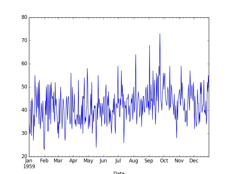
Daily Female Births Dataset
This dataset describes the number of daily female births in California in 1959.
The units are a count and there are 365 observations. The source of the dataset is credited to Newton (1988).
Running the example prints the first 5 rows of the dataset.
1
2
3
4
5
6
Date
1959-01-01 35
1959-01-02 32
1959-01-03 30
1959-01-04 31
1959-01-05 44
The series is then graphed as a line plot.
Daily Female Birth Dataset Line Plot
1. Select Time Series Forecast Model
You must select a model.
This is where the bulk of the effort will be in preparing the data, performing analysis, and ultimately selecting a model and model hyperparameters that best capture the relationships in the data.
In this case, we can arbitrarily select an autoregression model (AR) with a lag of 6 on the differenced dataset.
We can demonstrate this model below.
First, the data is transformed by differencing, with each observation transformed as:
1
value(t) = obs(t) - obs(t - 1)
Next, the AR(6) model is trained on 66% of the historical data. The regression coefficients learned by the model are extracted and used to make predictions in a rolling manner across the test dataset.
As each time step in the test dataset is executed, the prediction is made using the coefficients and stored. The actual observation for the time step is then made available and stored to be used as a lag variable for future predictions.
1
2
3
4
5
6
7
8
9
10
11
12
13
14
15
16
17
18
19
20
21
22
23
24
25
26
27
28
29
30
31
32
33
34
35
36
37
38
39
40
41
42
43
44
45
46
47
# fit and evaluate an AR model
from pandas import read_csv
from matplotlib import pyplot
from statsmodels.tsa.ar_model import AutoReg
from sklearn.metrics import mean_squared_error
import numpy
from math import sqrt
# create a difference transform of the dataset
def difference(dataset):
diff=list()
foriinrange(1,len(dataset)):
value=dataset[i]-dataset[i-1]
diff.append(value)
returnnumpy.array(diff)
# Make a prediction give regression coefficients and lag obs
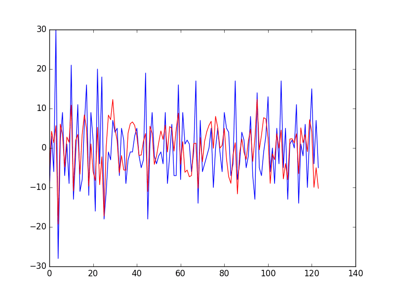
Running the example first prints the Root Mean Squared Error (RMSE) of the predictions, which is about 7 births on average.
This is how well we expect the model to perform on average when making forecasts on new data.
1
Test RMSE: 7.259
Finally, a graph is created showing the actual observations in the test dataset (blue) compared to the predictions (red).
Predictions vs Actual Daily Female Birth Dataset Line Plot
This may not be the very best possible model we could develop on this problem, but it is reasonable and skillful.
2. Finalize and Save Time Series Forecast Model
Once the model is selected, we must finalize it.
This means save the salient information learned by the model so that we do not have to re-create it every time a prediction is needed.
This involves first training the model on all available data and then saving the model to file.
The statsmodels implementations of time series models do provide built-in capability to save and load models by calling save() and load() on the fit AutoRegResults object.
For example, the code below will train an AR(6) model on the entire Female Births dataset and save it using the built-in save() function, which will essentially pickle the AutoRegResults object.
The differenced training data must also be saved, both the for the lag variables needed to make a prediction, and for knowledge of the number of observations seen, required by the predict() function of the AutoRegResults object.
Finally, we need to be able to transform the differenced dataset back into the original form. To do this, we must keep track of the last actual observation. This is so that the predicted differenced value can be added to it.
1
2
3
4
5
6
7
8
9
10
11
12
13
14
15
16
17
18
19
20
21
22
23
24
25
# fit an AR model and save the whole model to file
This code will create a file ar_model.pkl that you can load later and use to make predictions.
The entire training dataset is saved as ar_data.npy and the last observation is saved in the file ar_obs.npy as an array with one item.
The NumPy save() function is used to save the differenced training data and the observation. The load() function can then be used to load these arrays later.
The snippet below will load the model, differenced data, and last observation.
1
2
3
4
5
6
7
8
# load the AR model from file
from statsmodels.tsa.ar_model import AutoRegResults
import numpy
loaded=AutoRegResults.load('ar_model.pkl')
print(loaded.params)
data=numpy.load('ar_data.npy')
last_ob=numpy.load('ar_obs.npy')
print(last_ob)
Running the example prints the coefficients and the last observation.
I think this is good for most cases, but is also pretty heavy. You are subject to changes to the statsmodels API.
My preference is to work with the coefficients of the model directly, as in the case above, evaluating the model using a rolling forecast.
In this case, you could simply store the model coefficients and later load them and make predictions.
The example below saves just the coefficients from the model, as well as the minimum differenced lag values required to make the next prediction and the last observation needed to transform the next prediction made.
1
2
3
4
5
6
7
8
9
10
11
12
13
14
15
16
17
18
19
20
21
22
23
24
25
26
27
28
# fit an AR model and manually save coefficients to file
The coefficients are saved in the local file man_model.npy, the lag history is saved in the file man_data.npy, and the last observation is saved in the file man_obs.npy.
These values can then be loaded again as follows:
1
2
3
4
5
6
7
8
# load the manually saved model from file
import numpy
coef=numpy.load('man_model.npy')
print(coef)
lag=numpy.load('man_data.npy')
print(lag)
last_ob=numpy.load('man_obs.npy')
print(last_ob)
Running this example prints the loaded data for review. We can see the coefficients and last observation match the output from the previous example.
Now that we know how to save a finalized model, we can use it to make forecasts.
3. Make a Time Series Forecast
Making a forecast involves loading the saved model and estimating the observation at the next time step.
If the AutoRegResults object was serialized, we can use the predict() function to predict the next time period.
The example below shows how the next time period can be predicted.
The model, training data, and last observation are loaded from file.
The period is specified to the predict() function as the next time index after the end of the training data set. This index may be stored directly in a file instead of storing the entire training data, which may be an efficiency.
The prediction is made, which is in the context of the differenced dataset. To turn the prediction back into the original units, it must be added to the last known observation.
1
2
3
4
5
6
7
8
9
10
11
12
# load AR model from file and make a one-step prediction
from statsmodels.tsa.ar_model import AutoRegResults
We can also use a similar trick to load the raw coefficients and make a manual prediction.
The complete example is listed below.
1
2
3
4
5
6
7
8
9
10
11
12
13
14
15
16
17
18
# load a coefficients and from file and make a manual prediction
import numpy
def predict(coef,history):
yhat=coef[0]
foriinrange(1,len(coef)):
yhat+=coef[i]*history[-i]
returnyhat
# load model
coef=numpy.load('man_model.npy')
lag=numpy.load('man_data.npy')
last_ob=numpy.load('man_obs.npy')
# make prediction
prediction=predict(coef,lag)
# transform prediction
yhat=prediction+last_ob[0]
print('Prediction: %f'%yhat)
Running the example, we achieve the same prediction as we would expect, given the underlying model and method for making the prediction are the same.
1
Prediction: 46.755211
4. Update Forecast Model
Our work is not done.
Once the next real observation is made available, we must update the data associated with the model.
Specifically, we must update:
The differenced training dataset used as inputs to make the subsequent prediction.
The last observation, providing a context for the predicted differenced value.
Let’s assume the next actual observation in the series was 48.
The new observation must first be differenced with the last observation. It can then be stored in the list of differenced observations. Finally, the value can be stored as the last observation.
In the case of the stored AR model, we can update the ar_data.npy and ar_obs.npy files. The complete example is listed below:
1
2
3
4
5
6
7
8
9
10
11
12
13
14
# update the data for the AR model with a new obs
import numpy
# get real observation
observation=48
# load the saved data
data=numpy.load('ar_data.npy')
last_ob=numpy.load('ar_obs.npy')
# update and save differenced observation
diffed=observation-last_ob[0]
data=numpy.append(data,[diffed],axis=0)
numpy.save('ar_data.npy',data)
# update and save real observation
last_ob[0]=observation
numpy.save('ar_obs.npy',last_ob)
We can make the same changes for the data files for the manual case. Specifically, we can update the man_data.npy and man_obs.npy respectively.
The complete example is listed below.
1
2
3
4
5
6
7
8
9
10
11
12
13
# update the data for the manual model with a new obs
import numpy
# get real observation
observation=48
# update and save differenced observation
lag=numpy.load('man_data.npy')
last_ob=numpy.load('man_obs.npy')
diffed=observation-last_ob[0]
lag=numpy.append(lag[1:],[diffed],axis=0)
numpy.save('man_data.npy',lag)
# update and save real observation
last_ob[0]=observation
numpy.save('man_obs.npy',last_ob)
We have focused on one-step forecasts.
These methods would work just as easily for multi-step forecasts, by using the model repetitively and using forecasts of previous time steps as input lag values to predict observations for subsequent time steps.
Consider Storing All Observations
Generally, it is a good idea to keep track of all the observations.
This will allow you to:
Provide a context for further time series analysis to understand new changes in the data.
Train a new model in the future on the most recent data.
Back-test new and different models to see if performance can be improved.
For small applications, perhaps you could store the raw observations in a file alongside your model.
It may also be desirable to store the model coefficients and required lag data and last observation in plain text for easy review.
For larger applications, perhaps a database system could be used to store the observations.
Summary
In this tutorial, you discovered how to finalize a time series model and use it to make predictions with Python.
Specifically, you learned:
How to save a time series forecast model to file.
How to load a saved time series forecast from file and make a prediction.
How to update a time series forecast model with new observations.
Do you have any questions?
Ask your questions in the comments below and I will do my best to answer.
Want to Develop Time Series Forecasts with Python?
is it ok to apply time series analysis to predict patients status in ICU using ICU Database such as MIMIC II database? if it is then would be kind enough to guide me on this.
series = pd.read_csv(‘daily-total-female-births.csv’, header=0)
print(series.head())
series.plot()
plt.show()
I am not getting the same graph. The line graph appears more flat and the months are not showing. Was there additional codes not shown in the tutorial? Also, I tried using pyplot.show() so I update it to plt.show() and the code ran fine.
Confirm you have the latest version of Pandas and matplotlib installed. Also confirm that your data file contains date-times and observations with no additional data or footer information.
The additional data was deleted in the data file (thanks to your suggestion) and now the graph looks very similar, however the dates are missing. I’m assuming it’s because the indices are displayed on the x-axis. It was corrected once I set ‘Date’ as the index.
series=series.set_index(‘Date’)
The graph doesn’t look exactly like your graph but it’s close enough.
Hi Jason, Thank you so much for your nice examples.
I’ve been wasting my time playing with game results datasets and these first step into prediction was really handy. Usually, in these games there is no tendency at all, all balls have the same fair chance of getting out. How would you approach such predictions, for example for Euromillions?
Where can I find some more advanced time-series predictions for multivariate cases? I would like to predict the outcome of 3 variables that linked to each other. Similar code to this example would be perfect…
“These methods would work just as easily for multi-step forecasts, by using the model repetitively and using forecasts of previous time steps as input lag values to predict observations for subsequent time steps.”
Hello, Jason! I’m a little new to this forecasting modeling approach, and was able to successfully able to run your tutorial and examples no problem. However, as I’m still poking around to see how this works, is there a good example you could point to that explains your above quote? I get that the predict function looks at coef[0] to ultimately perform its calculation, and our forecasting approach provides the next time step’s prediction, but how do I tell the function “look at the NEXT time step after that one…” etc? Is it coef[1]…coef[n]?
Apologies if these are really dumb questions, I find this fascinating at how accurate it can be on even real world data, and want to do statistical analyses to find out when the “long term forecast” falls off a cliff when it comes to accuracy, I just haven’t been able to figure out how to ask for time steps farther away than 1.
Would you use the same method if you say, wanted to predict occupancy on a given floor, of a given building – provided you have time-series data of all of the login’s (and logoffs) of all occupants that come onto the floor – dating back say 1 or 2 years?
Also, would you use the same method if you wanted to “predict” this occupancy from NOW to say, 2 – 3 days in advance – for a specific day? how would the time-step look like for the next day or in 2 days?
Hello,
I will need your advice,
In fact, I have a large mass of data (almost 200 000), and I want to predict about 1 000 points.
Which algorithm would be most appropriate?
My database is univariate (just a data vector)
If you can direct me to a demo of “online prediction”, with real-time adaptation.
Hey,
I tried your code with your dataset, but i do not seem to be getting the same RMSE as your code. Is there any additional code you have missed out in your tutorial?
Dear Sir,
How can we plot graph with time as X-axis not the integers from csv file. If I directly read_csv file and plot then it works but after any type prediction model it always plot with integers values but I want Time as X-axis.
Thanks Sir in Advance
Lindsey Tran (Belliveau)July 22, 2020 at 10:41 am#
Hi Jason –
Would this be an issue if there wasn’t enough data?
I am stuck on the “maxlag should be < nobs" for a dataset of about 20 values.
Any pointers for how I can get around this?
Thank you and much appreciated!
Lindsey
I am using Weekly data for last 3 years (156 points) to check the forecast against the current years actuals which is 22 weeks. 178 points in total. If the model fits, i intend to use it for the following year. Data is seasonal as well. I guess i can run this code on Power BI to get the forecast for multiple sites(669 in total)?
If there is a dependent variable that has to be predicted and a datetime variable with no time information along with few categorical and numerical variables, can we split the date variable to day week, year month and drop the date column and predict the output , if so what type of variables will be the converted date time variable
Thanks for the good information on ARIMA.could you please let me know how to create a dataframe with actual and forecast and 95% confidence interval .waiting for your reply
Thanks for your good tutorial about time series forecasting.
Could you please tell me can time series data forecast in Support Vector Regression (SVR)?
I have followed your tutorial – once again. This time taking great care to copy the information.
My OS is Ubuntu 18.04
Vanilla install and everything updated.
I have created a Python3 environment and I have installed all the required module as required by your tutorial.
I have downloaded the dataset
This is the version of the modules I have installed.
scipy: 1.3.1
numpy: 1.17.0
matplotlib: 3.1.1
pandas: 0.25.1
sklearn: 0.21.3
statsmodels: 0.10.1
Dataset 93, Validation 12
When I execute your code I am confronted with an error.
File “complete.py”, line 47, in
X = X.astype(‘float32’)
ValueError: could not convert string to float: ‘1964-01’
Is it that the modules for this tutorial are older than the ones that I have installed or vise versa.
I could do with a bit of help. This is the only thing that is holding me back for purchasing your book.
Consider aggressively cutting the code back to the minimum required. This will help you isolate the problem and focus on it.
Consider cutting the problem back to just one or a few simple examples.
Consider finding other similar code examples that do work and slowly modify them to meet your needs. This might expose your misstep.
Consider posting your question and code to StackOverflow.
Hello,
let talk about the problem of prediction of user-preferred channel each hour(time series prediction problem). Suppose that I have many users, each user has his own list of channels. So each hour the user will watch a specific channel (each user has his own behavior). in my DB I have +40K users and almost 50 channels. Those 40K users are in fact the clusters for more than 60 Million users. So we can’t cluster anymore. I couldn’t find a way to build one model that predicts for each user, at a specific time, which channel that the user can watch. Per in mind that I solved the problem for one user (I mean based on the one user data, I build an LSTM model that predict the user preferred channel at a specific time). But the problem is generalized to 40K users. Should I build 40K models which mean model for each user !!, or there is alternative solution ?!
Firstly, it sounds like a classification problem, e.g. 50 channels are 50 classes. If you are modeling over time, it sounds like a time series classification problem.
You have lots of data, so I’d recommend testing a range of framing of the problem to see what works. E.g. model per customer, per customer group, across all customers, per day, per week, across all time, etc.
Then, we don’t know how hard the problem is so start with a naive model, compare to a linear model, some ml models, and even some deep learning models to see how learnable each framing happens to be.
Hello, I have managed to replicate your plots so far. However rather than plotting the actual and predicted birthrate difference (end of Section 1), I would like to plot the birthrate itself. How could I do that?
If we perform a Dickey-Fuller Test on the data, the results say the series is likely stationary. If this is the case, can we just do an AR on the actual data itself (i.e. do we need to do differencing)? If so, will this AR model on the actual data be enough, or do we also have to also model the residuals and include those in the predictions if there is a pattern is detected in the plot?
After performing the DF test and performing an AR on the data, I plotted the actual data and the yhat one. The yhat graph had very minor ups and downs (most of the data centered around 40 or 41) and in a way went through the actual data around the average (as if it were a straight line). It did not have the variability of the ups and downs that the differencing graph you had above. A test on the residuals failed the hypothesis that it was Gaussian.
I went ahead and modeled the residuals with lag15 and fixed the predictions based on the residual AR model. I ended up with a final model RMSE of 6.736 (vs 7.499 when you performed differencing on the data and fixed the forecasts with the residual AR model).
A test on the new residuals after performing the amended forecast also failed the normality test.
So, while I got a better RMSE, the errors are still do not have a normal distribution. Is this something to worry about and if so what do you recommend the next step be?
The next step is to continue to test data prep, models, model configs until you run out of time or ideas, or achieve good enough results/results that satisfy project stakeholders.
Hi sir…Hope so you are fine.
I am new to machine learning and i want to do future prediction of covid 19 cases from the previous cases using python. I need your suggestion from where i start and which features i have to chose. I will be highly thankful to you
This article is really helpful ! but i have oe question wanted to refer you. This is a deploymeny for LSTM model in flask python, i would like to further predict the near future value using the current value, its really stuck me quite for a while, please share me some tips ! Thanks in advance ~
app.py
from flask import Flask, make_response, request, render_template
from pandas import DataFrame
import io
from pandas import datetime
from io import StringIO
import csv
import pandas as pd
import numpy as np
import pickle
import os
from keras.models import load_model
from sklearn.preprocessing import MinMaxScaler
app = Flask(__name__)
@app.route(‘/’)
def form():
return “””
Let’s TRY to Predict..
Insert your CSV file and then download the Result
Predict
“””
@app.route(‘/transform’, methods=[“POST”])
def transform_view():
if request.method == ‘POST’:
f = request.files[‘data_file’]
if not f:
return “No file”
stream = io.StringIO(f.stream.read().decode(“UTF8”), newline=None)
csv_input = csv.reader(stream)
for row in csv_input:
print(row)
At the point where you do the graph, …..”Finally, a graph is created showing the actual observations in the test dataset (blue) compared to the predictions (red).”
Can you show us how can we graph the original non-differenced test data against the predictions at the same scale. I.e. graph the actual test data values vs. the actual predicted values.
Sambath Narayanan ParthasarathySeptember 3, 2022 at 4:50 pm#
Hello Jason, Thank you.Very rare piece of info with code. After detrending, removing seasonal effect, how does one get back orginal data in explainable form
This mapping also required for MAPE & RMSE?


Great Work sir.
is it ok to apply time series analysis to predict patients status in ICU using ICU Database such as MIMIC II database? if it is then would be kind enough to guide me on this.
Thanking you
It is not my area of expertise. It might be a fun learning exercise.
This process will guide you through your predictive modeling problem:
https://machinelearningmastery.com/start-here/#process
Hi there Shamsul. I wanna talk about your comment because I’m also working on this type of project.
Thanks for the tutorial.
I noticed that when I ran the following code:
series = pd.read_csv(‘daily-total-female-births.csv’, header=0)
print(series.head())
series.plot()
plt.show()
I am not getting the same graph. The line graph appears more flat and the months are not showing. Was there additional codes not shown in the tutorial? Also, I tried using pyplot.show() so I update it to plt.show() and the code ran fine.
Thanks for your help.
Hi Hoang,
There’s no additional code.
Confirm you have the latest version of Pandas and matplotlib installed. Also confirm that your data file contains date-times and observations with no additional data or footer information.
Thanks Jason, for your quick response.
I am using Pandas v0.19.2 and matplotlib v2.0.0.
The additional data was deleted in the data file (thanks to your suggestion) and now the graph looks very similar, however the dates are missing. I’m assuming it’s because the indices are displayed on the x-axis. It was corrected once I set ‘Date’ as the index.
series=series.set_index(‘Date’)
The graph doesn’t look exactly like your graph but it’s close enough.
Glad to hear you made some progress, thanks for providing the details. It may help others.
Hi Jason, Thank you so much for your nice examples.
I’ve been wasting my time playing with game results datasets and these first step into prediction was really handy. Usually, in these games there is no tendency at all, all balls have the same fair chance of getting out. How would you approach such predictions, for example for Euromillions?
Where can I find some more advanced time-series predictions for multivariate cases? I would like to predict the outcome of 3 variables that linked to each other. Similar code to this example would be perfect…
Thank you
Do you mean lotto? I believe that is random and not predictable.
Once you frame your time series as a supervised learning problem, you can use a suite of machine learning methods.
For predicting 3 variables, I would recommend a neural network model.
Hi Jason,
Great content as always.
I had a question.
1) Why did you not use ARIMA model here and why AR? Is there a difference?
There is a difference, AR does not include the differencing and moving average. It’s a simpler method.
It is just an example for making predictions, you could swap in ARIMA if you like.
Hi Jason,
Really good stuff!
# make prediction
predictions = model.predict(start=len(data), end=len(data))
here the minimum value for start should be window (6 in this case) and less than the end time.
Thanks Martha.
“These methods would work just as easily for multi-step forecasts, by using the model repetitively and using forecasts of previous time steps as input lag values to predict observations for subsequent time steps.”
Hello, Jason! I’m a little new to this forecasting modeling approach, and was able to successfully able to run your tutorial and examples no problem. However, as I’m still poking around to see how this works, is there a good example you could point to that explains your above quote? I get that the predict function looks at coef[0] to ultimately perform its calculation, and our forecasting approach provides the next time step’s prediction, but how do I tell the function “look at the NEXT time step after that one…” etc? Is it coef[1]…coef[n]?
Apologies if these are really dumb questions, I find this fascinating at how accurate it can be on even real world data, and want to do statistical analyses to find out when the “long term forecast” falls off a cliff when it comes to accuracy, I just haven’t been able to figure out how to ask for time steps farther away than 1.
It is a good question.
You can use the model recursively but taking the forecast and using it as an observation in order to make the next forecast.
This post might have more details on the topic:
https://machinelearningmastery.com/multi-step-time-series-forecasting/
Jason – awesome example.
Would you use the same method if you say, wanted to predict occupancy on a given floor, of a given building – provided you have time-series data of all of the login’s (and logoffs) of all occupants that come onto the floor – dating back say 1 or 2 years?
Also, would you use the same method if you wanted to “predict” this occupancy from NOW to say, 2 – 3 days in advance – for a specific day? how would the time-step look like for the next day or in 2 days?
Perhaps. Try it and see how it performs on your data.
This is a great tutorial. I have a question why did you transform the data?
And why using difference ?
Is it necessary to transform the data ?
The data had a trend, I removed it via differencing.
Learn more about differencing here:
https://machinelearningmastery.com/remove-trends-seasonality-difference-transform-python/
How can I check the prediction performance
You can calculate the error between predictions and actual values.
Hello,
I will need your advice,
In fact, I have a large mass of data (almost 200 000), and I want to predict about 1 000 points.
Which algorithm would be most appropriate?
My database is univariate (just a data vector)
If you can direct me to a demo of “online prediction”, with real-time adaptation.
I recommend that you follow this process:
https://machinelearningmastery.com/how-to-develop-a-skilful-time-series-forecasting-model/
Hey,
I tried your code with your dataset, but i do not seem to be getting the same RMSE as your code. Is there any additional code you have missed out in your tutorial?
Thanks
~M
Perhaps some of these suggestions will help:
https://machinelearningmastery.com/faq/single-faq/why-does-the-code-in-the-tutorial-not-work-for-me
Dear Sir,
How can we plot graph with time as X-axis not the integers from csv file. If I directly read_csv file and plot then it works but after any type prediction model it always plot with integers values but I want Time as X-axis.
Thanks Sir in Advance
This post will help you get started with plotting:
https://machinelearningmastery.com/data-visualization-methods-in-python/
HI Jason ,
Not sure how do i fix the following error
maxlag should be 27 model_fit = model.fit(maxlag=6,disp=False)
maxlag should be < nobs
Yes.
Perhaps it is related to the amount of data used to fit the model?
Hi Jason –
Would this be an issue if there wasn’t enough data?
I am stuck on the “maxlag should be < nobs" for a dataset of about 20 values.
Any pointers for how I can get around this?
Thank you and much appreciated!
Lindsey
Not sure what you mean by “get around this” sorry.
Maybe this will help:
https://machinelearningmastery.com/time-series-forecasting-supervised-learning/
No problem 🙂
I mean how can I fix this issue for my dataset.
I will take a look at this link, thank you!
Sure, set the lag to anything you like.
Sorry, perhaps I don’t understand the problem you’re having and how I can help.
Hi Jason,
Thanks for responding. I am struggling here.
I am using Weekly data for last 3 years (156 points) to check the forecast against the current years actuals which is 22 weeks. 178 points in total. If the model fits, i intend to use it for the following year. Data is seasonal as well. I guess i can run this code on Power BI to get the forecast for multiple sites(669 in total)?
Good question about multiple sites, you have many options.
This might give you some ideas:
https://machinelearningmastery.com/faq/single-faq/how-to-develop-forecast-models-for-multiple-sites
Hi Sir ,
Just a basic question here why are substracting the value from previous ones ?
Doesn’t the algorithm find the patter and help us in predictions?
Also sir my r2 value is .35 will that ok or should i work further ?
Really sorry if that was a very bad question but I’m new here so asked
Thanks
It is called differencing and it removes the trend, more here:
https://machinelearningmastery.com/difference-time-series-dataset-python/
If there is a dependent variable that has to be predicted and a datetime variable with no time information along with few categorical and numerical variables, can we split the date variable to day week, year month and drop the date column and predict the output , if so what type of variables will be the converted date time variable
Typically we drop the date/time variable once the data has a consistent interval/spacing.
Hi Jason,
Thanks for the good information on ARIMA.could you please let me know how to create a dataframe with actual and forecast and 95% confidence interval .waiting for your reply
Regards
Prakash Hullathi
Here is an example of calculating a predicting interval with ARIMA:
https://machinelearningmastery.com/time-series-forecast-uncertainty-using-confidence-intervals-python/
Hai Jason,
Thanks for your good tutorial about time series forecasting.
Could you please tell me can time series data forecast in Support Vector Regression (SVR)?
Yes, I don’t see why not.
do you have tutorial about it?
Yes, this might help:
https://machinelearningmastery.com/multi-step-time-series-forecasting-with-machine-learning-models-for-household-electricity-consumption/
thank you
I have followed your tutorial – once again. This time taking great care to copy the information.
My OS is Ubuntu 18.04
Vanilla install and everything updated.
I have created a Python3 environment and I have installed all the required module as required by your tutorial.
I have downloaded the dataset
This is the version of the modules I have installed.
scipy: 1.3.1
numpy: 1.17.0
matplotlib: 3.1.1
pandas: 0.25.1
sklearn: 0.21.3
statsmodels: 0.10.1
Dataset 93, Validation 12
When I execute your code I am confronted with an error.
File “complete.py”, line 47, in
X = X.astype(‘float32’)
ValueError: could not convert string to float: ‘1964-01’
Is it that the modules for this tutorial are older than the ones that I have installed or vise versa.
I could do with a bit of help. This is the only thing that is holding me back for purchasing your book.
Yes the API has changed.
I have updated all examples in the tutorial.
Thanks.
ValueError: end is before start
Im getting this error while trying to find the prediction for observation =48.
Do u have any solution?
I have some suggestions here that may help:
Consider aggressively cutting the code back to the minimum required. This will help you isolate the problem and focus on it.
Consider cutting the problem back to just one or a few simple examples.
Consider finding other similar code examples that do work and slowly modify them to meet your needs. This might expose your misstep.
Consider posting your question and code to StackOverflow.
Hello,
let talk about the problem of prediction of user-preferred channel each hour(time series prediction problem). Suppose that I have many users, each user has his own list of channels. So each hour the user will watch a specific channel (each user has his own behavior). in my DB I have +40K users and almost 50 channels. Those 40K users are in fact the clusters for more than 60 Million users. So we can’t cluster anymore. I couldn’t find a way to build one model that predicts for each user, at a specific time, which channel that the user can watch. Per in mind that I solved the problem for one user (I mean based on the one user data, I build an LSTM model that predict the user preferred channel at a specific time). But the problem is generalized to 40K users. Should I build 40K models which mean model for each user !!, or there is alternative solution ?!
Great question.
Firstly, it sounds like a classification problem, e.g. 50 channels are 50 classes. If you are modeling over time, it sounds like a time series classification problem.
You have lots of data, so I’d recommend testing a range of framing of the problem to see what works. E.g. model per customer, per customer group, across all customers, per day, per week, across all time, etc.
Then, we don’t know how hard the problem is so start with a naive model, compare to a linear model, some ml models, and even some deep learning models to see how learnable each framing happens to be.
Does that help?
Hi Jason,
thanks for you post.
I want to ask if there is example about long-term time series prediction based on LSTM model?
by direct prediction method or recurrent method?
Looking forward to your reply!
Best regards
Hao
Yes, this will help:
https://machinelearningmastery.com/faq/single-faq/how-do-you-use-lstms-for-multi-step-time-series-forecasting
Hello, I have managed to replicate your plots so far. However rather than plotting the actual and predicted birthrate difference (end of Section 1), I would like to plot the birthrate itself. How could I do that?
You can call pyplot.plot() and pass in any data you want.
Hey,
After updating the data, now how to again predict the values?
now what will be the prediction values?
can i have updating prediction value code?
You can call predict() or forecast() directly on your model as described in the above tutorial.
can I use this code for predict future sales restaurant?
Perhaps try it and see if it is appropriate for your dataset.
Hi Jason,
If we perform a Dickey-Fuller Test on the data, the results say the series is likely stationary. If this is the case, can we just do an AR on the actual data itself (i.e. do we need to do differencing)? If so, will this AR model on the actual data be enough, or do we also have to also model the residuals and include those in the predictions if there is a pattern is detected in the plot?
Yes, try it and compare results to the same dataset with differencing.
Hi Jason,
After performing the DF test and performing an AR on the data, I plotted the actual data and the yhat one. The yhat graph had very minor ups and downs (most of the data centered around 40 or 41) and in a way went through the actual data around the average (as if it were a straight line). It did not have the variability of the ups and downs that the differencing graph you had above. A test on the residuals failed the hypothesis that it was Gaussian.
I went ahead and modeled the residuals with lag15 and fixed the predictions based on the residual AR model. I ended up with a final model RMSE of 6.736 (vs 7.499 when you performed differencing on the data and fixed the forecasts with the residual AR model).
A test on the new residuals after performing the amended forecast also failed the normality test.
So, while I got a better RMSE, the errors are still do not have a normal distribution. Is this something to worry about and if so what do you recommend the next step be?
Perhaps not.
The next step is to continue to test data prep, models, model configs until you run out of time or ideas, or achieve good enough results/results that satisfy project stakeholders.
Hi sir…Hope so you are fine.
I am new to machine learning and i want to do future prediction of covid 19 cases from the previous cases using python. I need your suggestion from where i start and which features i have to chose. I will be highly thankful to you
See this:
https://machinelearningmastery.com/faq/single-faq/how-can-i-use-machine-learning-to-model-covid-19-data
This article is really helpful ! but i have oe question wanted to refer you. This is a deploymeny for LSTM model in flask python, i would like to further predict the near future value using the current value, its really stuck me quite for a while, please share me some tips ! Thanks in advance ~
app.py
from flask import Flask, make_response, request, render_template
from pandas import DataFrame
import io
from pandas import datetime
from io import StringIO
import csv
import pandas as pd
import numpy as np
import pickle
import os
from keras.models import load_model
from sklearn.preprocessing import MinMaxScaler
app = Flask(__name__)
@app.route(‘/’)
def form():
return “””
Let’s TRY to Predict..
Insert your CSV file and then download the Result
Predict
“””
@app.route(‘/transform’, methods=[“POST”])
def transform_view():
if request.method == ‘POST’:
f = request.files[‘data_file’]
if not f:
return “No file”
stream = io.StringIO(f.stream.read().decode(“UTF8”), newline=None)
csv_input = csv.reader(stream)
for row in csv_input:
print(row)
stream.seek(0)
result = stream.read()
df = pd.read_csv(StringIO(result), usecols=[1])
df2 = pd.read_csv(StringIO(result))
matrix2 = df2[df2.columns[0]].to_numpy()
list1 = matrix2.tolist()
# load the model from disk
model = load_model(‘model.h5’)
dataset = df.values
dataset = dataset.astype(‘float32’)
scaler = MinMaxScaler(feature_range=(0, 1))
dataset = scaler.fit_transform(dataset)
dataset = np.reshape(dataset, (dataset.shape[0], 1, dataset.shape[1]))
predict = model.predict(dataset)
transform = scaler.inverse_transform(predict)
dataFrame = DataFrame()
dataFrame[‘Month’] = list1
dataFrame[‘predicted value’] = transform
##df_predict = pd.DataFrame(transform, columns=[“predicted value”])
response = make_response(dataFrame.to_csv(index = False, encoding=’utf8′))
response.headers[“Content-Disposition”] = “attachment; filename=result.csv”
return response
if __name__ == “__main__”:
app.run(debug=True, port = 9000, host = “localhost”)
Sorry, I don’t have the capacity to review your code for you.
perhaps can you share with me some source regarding this issues ?
Very nice article! Thank you.
At the point where you do the graph, …..”Finally, a graph is created showing the actual observations in the test dataset (blue) compared to the predictions (red).”
Can you show us how can we graph the original non-differenced test data against the predictions at the same scale. I.e. graph the actual test data values vs. the actual predicted values.
Thank you
You’re welcome.
Yes, you can use matplotlib to create line plots, this is a good starting point:
https://machinelearningmastery.com/time-series-data-visualization-with-python/
how to plot observed data (train) with forecast data values in same figure.
the two series are plotted from beginning 0 value not contentiously
Hello Hala…Try this method:
https://www.kite.com/python/answers/how-to-make-multiple-plots-on-the-same-figure-in-matplotlib-in-python
Hello Jason, Thank you.Very rare piece of info with code. After detrending, removing seasonal effect, how does one get back orginal data in explainable form
This mapping also required for MAPE & RMSE?
Am I right? how to go about?
Hi Sambath…You may find the following of interest:
https://www.machinelearningplus.com/time-series/time-series-analysis-python/